


Models of valves.


Flow and Pressure Control Valves
--------------------------------

These valves control the flow or pressure. They are modelled as static systems.
Every valve has lumped volumes connected at every port.

CheckValve:	Ideal spring-loaded check valve with laminar/turbulent flow.
CheckValveTwo:	Ideal spring-loaded check valve with laminar/turbulent flow
		(different characteristics).
ShuttleValve:	Ideal Shuttle valve with internal resistance (static model).
ReducingValve:	Ideal pressure reducing valve (static model).
SerFlowCont:	Ideal series flow control valve (static model).


Spool Valves
------------

These valves control the flow according to the position of the spool. The spool dynamics is
modelled as a second order system with limits for the spool velocity and position. Every valve
has lumped volumes connected at every port.

ServoValve:	Valve with second order spool dynamics and nonlinearities. Flow area depends
		linearly on spool position.
PropValve:	Valve with second order spool dynamics and nonlinearities. Flow area depends
		not linearly on spool position, usually large overlap.


Release Notes:
--------------

1999 - 10 - 9: coded
 HyLibLight.Components.ReliefValve
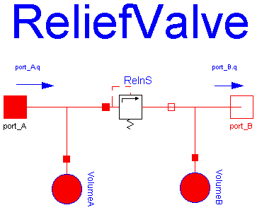
Static model of a relief valve.

The resistance depends on the pressure differential
   dp = port_A.p - port_B.p

1) dp < pclosed => valve closed, only leakage
                   q = dp * GLeak

2) pclosed < dp < popen => working range,
                           i. e. valve partially opened

3) popen < dp => valve wide open, q = dp * GOpen

Use the modifier(s)

   VolumeA(port_A(p(start=1e5)))
and/or
   VolumeB(port_A(p(start=1e5)))

to set initial condition(s) for the pressure of the lumped volume(s) [Pa].

If a state is deselected by Dymola during the index reduction process this
modifier has no effect.

Release Notes:
--------------

2000 - 2 - 7: tested
| Name | Default | Description |
|---|---|---|
| pclosed | 190e5 | valve closed if dp smaller [Pa] |
| popen | 205e5 | valve wide open if dp higher [Pa] |
| GLeak | 1.111e-12 | conductance of leakage of closed valve [m3/(s*Pa)] |
| GOpen | 1.666e-9 | conductance of wide open valve [m3/(s*Pa)] |
| volumeA | 1e-6 | volume at port A [m3] |
| volumeB | 1e-6 | volume at port B [m3] |
model ReliefValve "Static model of a relief valve."
  extends HyLibLight.Interfaces.TwoPortSys;
  parameter Modelica.SIunits.Pressure pclosed=190e5
    "valve closed if dp smaller";
  parameter Modelica.SIunits.Pressure popen=205e5
    "valve wide open if dp higher";
  parameter HyLibLight.Interfaces.HyLibUnits.Conductance GLeak=1.111e-12
    "conductance of leakage of closed valve";
  parameter HyLibLight.Interfaces.HyLibUnits.Conductance GOpen=1.666e-9
    "conductance of wide open valve";
  parameter Modelica.SIunits.Volume volumeA=1e-6 "volume at port A";
  parameter Modelica.SIunits.Volume volumeB=1e-6 "volume at port B";

  HyLibLight.Components.Basic.ReliefValveNoStates RelnS(
    pclosed=pclosed,
    popen=popen,
    GLeak=GLeak,
    GOpen=GOpen);
  HyLibLight.Components.VolumeConst VolumeA(volume=volumeA);
  HyLibLight.Components.VolumeConst VolumeB(volume=volumeB);
equation
  connect(RelnS.port_B, port_B);
  connect(port_A, RelnS.port_A);
  connect(VolumeA.port_A, RelnS.port_A);
  connect(RelnS.port_B, VolumeB.port_A);
end ReliefValve;
 HyLibLight.Components.CheckValve
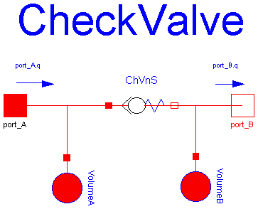
Spring-loaded check valve with laminar/turbulent flow.

The resistance depends on the pressure differential

1) pressure differential dp < p_closed
    => q = dp * GLeak
       leakage from high pressure port to low pressure port only

2) p_closed < dp < p_open
    => valve is partially open

3) dp > p_open
    => valve is wide open,
       flow mode depends on Reynolds number
       resistance modelled as orifice parallel with laminar resistance (leakage)

       The mass and flow forces are not included.

Use the modifier(s)

   VolumeA(port_A(p(start=1e5)))
and/or
   VolumeB(port_A(p(start=1e5)))

to set initial condition(s) for the pressure of the lumped volume(s) [Pa].

If a state is deselected by Dymola during the index reduction process this
modifier has no effect.


Release Notes:
--------------

2000 - 2 - 4: tested
| Name | Default | Description |
|---|---|---|
| pclosed | 1e5 | pressure to start opening the valve [Pa] |
| popen | 1.25e5 | pressure to open valve completely [Pa] |
| diameter | 1.e-3 | diameter of equivalent orifice [m] |
| k1 | 10. | laminar part [ ] |
| k2 | 2. | tubulent part, k2 = 1 / C_d^2 [ ] |
| GLeak | 1.e-12 | conductance of leakage [m3/(s*Pa)] |
| volumeA | 1e-6 | volume at port A [m3] |
| volumeB | 1e-6 | volume at port B [m3] |
model CheckValve
  "Spring-loaded check valve with laminar/turbulent flow."
  extends HyLibLight.Interfaces.TwoPortSys;
  parameter Modelica.SIunits.Pressure pclosed=1e5
    "pressure to start opening the valve";
  parameter Modelica.SIunits.Pressure popen=1.25e5
    "pressure to open valve completely";
  parameter Modelica.SIunits.Diameter diameter=1.e-3
    "diameter of equivalent orifice";
  parameter Real k1=10. "laminar part [ ]";
  parameter Real k2=2. "tubulent part, k2 = 1 / C_d^2 [ ]";
  parameter HyLibLight.Interfaces.HyLibUnits.Conductance GLeak=1.e-12
    "conductance of leakage";
  parameter Modelica.SIunits.Volume volumeA=1e-6 "volume at port A";
  parameter Modelica.SIunits.Volume volumeB=1e-6 "volume at port B";

  HyLibLight.Components.Basic.CheckValveNoStates ChVnS(
    pclosed=pclosed,
    popen=popen,
    diameter=diameter,
    k1=k1,
    k2=k2,
    GLeak=GLeak);
  HyLibLight.Components.VolumeConst VolumeA(volume=volumeA);
  HyLibLight.Components.VolumeConst VolumeB(volume=volumeB);
equation
  connect(ChVnS.port_B, port_B);
  connect(port_A, ChVnS.port_A);
  connect(VolumeA.port_A, ChVnS.port_A);
  connect(ChVnS.port_B, VolumeB.port_A);
end CheckValve;
 HyLibLight.Components.VolumeConst

Lumped volume with constant bulk modulus.

The pressure in the volume is calculated by:

d port_A.p     beta
---------- = -------- * port_A.q(t)
d Time        volume

with: 	port_A.p pressure in the volume
	beta	 bulk modulus in Pa (constant, default beta=1.6e9 Pa)
	volume	 volume of oil under pressure in m^3 (constant)
	port_A.q flow rate into the volume

If the calculated pressure falls below the vapour pressure
the pressure port_A.p is NOT limited to the vapour pressure.

To set the initial condition, i. e. the pressure in the lumped volume at
simulation start, to e. g. 2e6 Pa use the modifier:

	port_A(p(start=2e6))

If this state is deselected by Dymola during the index reduction process this
modifier has no effect.

See also:
Volume 		Volume with pressure dependent bulk modulus
VolumeTemp	Volume with pressure and temperature dependent bulk modulus


Release Notes:
--------------

1999 - 1 - 24: tested
| Name | Default | Description |
|---|---|---|
| volume | 1e-6 | volume [m3] |
| beta | 1.6e9 | effective bulk modulus [Pa] |
model VolumeConst "Lumped volume with constant bulk modulus."
  extends Components.Basic.VolumePartial;
  parameter Modelica.SIunits.Volume volume(final min=HyLibLight.Interfaces.
        FluidProp.VolMin) = 1e-6 "volume";
  parameter Modelica.SIunits.BulkModulus beta=1.6e9
    "effective bulk modulus";
equation
  der(port_A.p) = beta/volume*port_A.q;
end VolumeConst;
 HyLibLight.Components.LamRes
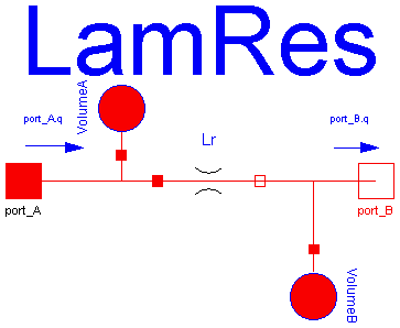
LamRes describes the laminar flow through a resistance
that has lumped volumes at each port.

q = G*dp

q   flow rate
G   conductance, m^3/(s * Pa)
dp  pressure drop across resistance

Equations to calculate the conductance G are given in the manual
for several components. A conductance of G = 4.167e-13 m^3/s/Pa
leads to a flow rate of 1 l/min at 4e7 Pa (=400 bar).

As the critical Reynolds number depends on the component there is
no check whether the flow is actually laminar or turbulent.

Use the modifier(s)

   VolumeA(port_A(p(start=1e5)))
and/or
   VolumeB(port_A(p(start=1e5)))

to set initial condition(s) for the pressure of the lumped volume(s) [Pa].

If a state is deselected by Dymola during the index reduction process this
modifier has no effect.

See also:

Orifice:	The model based on the loss coefficient K describes both flow regimes,
		laminar for very small Reynolds numbers, turbulent for higher
		Reynolds numbers (default model).
OriPoly:	The model describes both flow regimes, using a interpolation polynomial.
OriCav:		Orifice model checking for cavitation.
SimOri:		Texbook model, using a constant discharge coefficient
		(valid for turbulent flow only).
MeteringOri:	Metering Orifice, i. e. model OrificeNoStates with variable diameter.
TwoOrifices:	Two orifices in series, one with variable the other with
		fixed flow area.


Release Notes:
--------------

1999 - 10 - 23: tested
| Name | Default | Description |
|---|---|---|
| G | 4.2e-13 | conductance of laminar resistance [m3/(s*Pa)] |
| volumeA | 1.e-6 | volume at port A [m3] |
| volumeB | 1.e-6 | volume at port B [m3] |
model LamRes "Resistance with laminar flow and volumes at the ports."

  extends HyLibLight.Interfaces.TwoPortSys;
  parameter HyLibLight.Interfaces.HyLibUnits.Conductance G=4.2e-13
    "conductance of laminar resistance";
  parameter Modelica.SIunits.Volume volumeA=1.e-6 "volume at port A"
    ;
  parameter Modelica.SIunits.Volume volumeB=1.e-6 "volume at port B"
    ;
  HyLibLight.Components.Basic.LamResNoStates Lr(G=G);
  HyLibLight.Components.VolumeConst VolumeA(volume=volumeA);
  HyLibLight.Components.VolumeConst VolumeB(volume=volumeB);
equation
  connect(Lr.port_B, port_B);
  connect(Lr.port_A, port_A);
  connect(VolumeA.port_A, port_A);
  connect(VolumeB.port_A, port_B);
end LamRes;
 HyLibLight.Components.QMeas
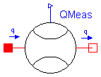
Measures the connector-flow rate between two ports in an ideal way
and provides the result as output signal outPort.signal[1] = q
(to be further processed with blocks of the Modelica.Blocks library).

Release Notes:
--------------

2000 - 1 - 24: tested
model QMeas "Flow rate sensor"
  HyLibLight.Interfaces.Port_A port_A
    "Port A, were oil flows into the component (positive q, port_A.p > port_B.p means positive dp)"
    ;
  HyLibLight.Interfaces.Port_B port_B
    "Port B, were oil leaves the component (negative q, port_A.p > port_B.p means positive dp)"
    ;
  Modelica.Blocks.Interfaces.OutPort outPort(final n=1);
equation

  outPort.signal[1] = port_A.q;
  port_A.q + port_B.q = 0;
  port_A.p = port_B.p;
end QMeas;
 HyLibLight.Components.PMeas
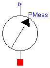
Measures the pressure p at port in an ideal way and provides the
result as output signal outPort.signal[1]
(to be further processed with blocks of the Modelica.Blocks library).

Release Notes:
--------------

2000 - 1 - 24: tested
model PMeas "Pressure sensor"
  HyLibLight.Interfaces.Port_A port_A
    "Port A, were oil flows into the component (positive q, port_A.p > port_B.p means positive dp)"
    ;
  Modelica.Blocks.Interfaces.OutPort outPort(final n=1);
equation
  port_A.q = 0;
  port_A.p = outPort.signal[1];
end PMeas;
 HyLibLight.Components.LongLine
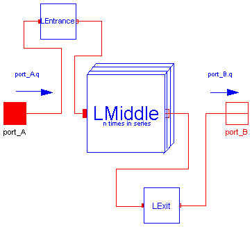
Dynamic model of a long line with compressibility, inductance
and frequency dependent viscosity.

This model uses n elements for the line =>
          ElementLength = line length / n

The oil in long lines is compressible, has a mass and a resistance.
The model includes the frequency dependent friction, compressibility
and inductance.

The dynamic response of long lines is a function of time and the spatial
coordinate, i. e. described by partial differential equations. For the
library a lumped parameter model is used that breaks the whole line into
n short elements. LongLine uses an entrance and an exit element that have
only half the length of the n-1 middle elements, leading to an effective
element length of 1 / n of the whole line length.

				      aSound
The model is adequate if: length < --------------
				    10 * fmax

		with	length  length of line segment
			aSound	speed of sound in fluid
			fmax 	highest frequency of interest

The steady state flow rate q is positive if oil enters the line at port_A,
the pressure drop port_A.p - port_B.p is then positive.

The resistance, compressibility, inductance and frequency
dependent viscosity are modelled.

The model is valid if the flow is laminar. There is no warning
if this condition is not met. The Reynolds number is computed for
the entrance and the exit element (to reduce the neccessary computations).


Release Notes:
--------------

2000 - 1 - 17: tested
| Name | Default | Description |
|---|---|---|
| LineLength | 31.98 | total length of line [m] |
| n | 10 | number of line segments |
| ElementLength | LineLength/n | length of one segment of line [m] |
| diameter | 30.e-3 | line diameter [m] |
| aSound | 1335 | speed of sound in oil [m/s] |
model LongLine "Long line with laminar flow"
  extends HyLibLight.Interfaces.TwoPortSys;
  parameter Modelica.SIunits.Length LineLength=31.98
    "total length of line";
  parameter Integer n(final min=2) = 10 "number of line segments";
  parameter Modelica.SIunits.Length ElementLength=LineLength/n
    "length of one segment of line";
  parameter Modelica.SIunits.Diameter diameter=30.e-3
    "line diameter";
  parameter Modelica.SIunits.VelocityOfSound aSound=1335
    "speed of sound in oil";
  HyLibLight.Components.Basic.LineMiddle[n - 1] LMiddle(
    ElementLength=ElementLength,
    diameter=diameter,
    aSound=aSound);

  HyLibLight.Components.Basic.LineEntrance LEntrance(
    ElementLength=ElementLength,
    diameter=diameter,
    aSound=aSound);
  HyLibLight.Components.Basic.LineExit LExit(
    ElementLength=ElementLength,
    diameter=diameter,
    aSound=aSound);
equation
  connect(LExit.port_B, port_B);
  connect(port_A, LEntrance.port_A);
  for i in 1:(n - 2) loop
    connect(LMiddle[i].port_B, LMiddle[i + 1].port_A);
  end for;

  connect(LEntrance.port_B, LMiddle[1].port_A);
  connect(LMiddle[n - 1].port_B, LExit.port_A);
end LongLine;