ObjectStab.Loads

Information

The loads subpackage contains definitions of various load models.

ObjectStab.Loads.PQLoad

Information

For a constant power the actual load powers drawn from the network 
are given by:

  Pl = P0
  Ql = Q0

Parameters

Name	Default	Description
P0	1	Rated Load Active Power (at 1 p.u. voltage) [p.u.]
Q0	0.2	Rated Load Reactive Power [p.u.]

Modelica definition

model PQLoad "Constant power (PQ) Load" 
  extends Partials.Load;
equation 
  Pl = P0;
  Ql = Q0;
end PQLoad;

ObjectStab.Loads.InductionMachine

Information

The induction motor load model is modelled by a transient EMF behind a 
transient reactance according to [1, pp. 376-378]. 

The load torque characteristic is given by parameters A,B and C:

  Tm = P0*(w*w/ws^2*A + B*w/ws + C)

where ws is the rated angular frequency.

Note that the parameter Q0 is not used. The reactive power drawn by the 
induction motor load is implicitly determined by the motor operating point.

---
[1] J. Machowski, J.W. Bialek, and J.R. Bumby, Power System Dynamics and 
Stability, Number ISBN 0-471-97174. Wiley, 1993.

Parameters

Name	Default	Description
P0	1	Rated Load Active Power (at 1 p.u. voltage) [p.u.]
Q0	0.2	Rated Load Reactive Power [p.u.]
rs	0.00438	Stator Resistance [p.u.]
xs	0.15	Stator Reactance [p.u.]
rr	0.25	Rotor Resistance [p.u.]
xr	0.01	Rotor Reactance [p.u.]
xm	2.60	Magnetizing Reactance [p.u.]
H	1	Inertia Constant [s]
A	1	Load Torque Characterstics - A
B	0	Load Torque Characterstics - B
C	0	Load Torque Characterstics - C
x	xs + xm	No-load reactance (calculated) [p.u.]
xp	xs + xr*xm/(xr + xm)	Transient Reactance (calculated) [p.u.]
T0p	(xr + xm)/(Base.ws*rr)	Transient no-load time constant (calculated) [s]

Modelica definition

model InductionMachine "Induction machine load model" 
  extends Partials.Load;
  parameter Base.Resistance rs=0.00438 "Stator Resistance";
  parameter Base.Reactance xs=0.15 "Stator Reactance";
  parameter Base.Resistance rr=0.25 "Rotor Resistance";
  parameter Base.Reactance xr=0.01 "Rotor Reactance";
  parameter Base.Reactance xm=2.60 "Magnetizing Reactance";
  parameter Base.InertiaConstant H=1 "Inertia Constant";
  parameter Real A=1 "Load Torque Characterstics - A";
  parameter Real B=0 "Load Torque Characterstics - B";
  parameter Real C=0 "Load Torque Characterstics - C";
  parameter Base.Reactance x=xs + xm 
    "No-load reactance (calculated)";
  parameter Base.Reactance xp=xs + xr*xm/(xr + xm) 
    "Transient Reactance (calculated)";
  parameter Base.Time T0p=(xr + xm)/(Base.ws*rr) 
    "Transient no-load time constant (calculated)";
  
  Real s "slip";
  Base.VoltageRealPart Eap(start=1) 
    "Real part of transient EMF [p.u.]";
  Base.VoltageImagPart Ebp "Imaginary part of transient EMF [p.u.]";
  Base.ElectricalTorque Te "Electrical torque [p.u.]";
  Base.MechanicalTorque Tm "Load mechanical torque [p.u.]";
  Base.AngularVelocity w "Angular speed [rad/s]";
equation 
  // stator equations
  [T.vb; T.va + 1] = [Ebp; Eap] + [rs, xp; -xp, rs]*[T.ib; T.ia];
  
  // EMF equations
  der(Ebp) = -s*Base.ws*Eap - (Ebp - (x - xp)*T.ia)/T0p;
  der(Eap) = s*Base.ws*Ebp - (Eap + (x - xp)*T.ib)/T0p;
  
  // generated electrical torque
  Te = Ebp*T.ib + Eap*T.ia;
  
  // inertia equation 
  2*H/Base.ws*der(w) = Te - Tm;
  
  // slip equation
  s = (Base.ws - w)/Base.ws;
  
  // load torque characteristic
  Tm = P0*(w*w/Base.ws/Base.ws*A + B*w/Base.ws + C);
end InductionMachine;

ObjectStab.Loads.DynLoad

Information

Dynamic exponential recovery load according to Karlsson & Hill [1].

The load powers are given by:

  der(xp) = P0*(V^(as) - V^at) - xp/Tp;
  Pl = (xp/Tp + P0*V^at);
  der(xq) = Q0*(V^(bs) - V^bt) - xq/Tq;
  Ql = (xq/Tq + Q0*V^bt);

where xp is a continuous dynamic state that can be interpreted as a
measure of the energy deficit in the load and Ps(V) = P0*V^as 
is the steady-state and Pt(V)=P0*V^at the transient voltage dependency.
Pl is the actual active load power and Tp is the active power recovery 
time constant. 

For the reactive load power, a similar model is used with corresponding 
characteristics x_q, Qs(V)=Q0 V^bs, Qt(V) = Q0 V^bt and time constant Tq.

---
[1] D. Karlsson and D.J. Hill, "Modelling and identification of nonlinear 
dynamic loads in power systems", IEEE Transactions on Power Systems, 
vol. 9, no. 1, pp. 157-163, February 1994.

Parameters

Name	Default	Description
P0	1	Rated Load Active Power (at 1 p.u. voltage) [p.u.]
Q0	0.2	Rated Load Reactive Power [p.u.]
as	0	Steady-state active power voltage dependency
at	2	Transient active power voltage dependency
bs	0	Steady-state reactive power voltage dependency
bt	2	Transient reactive power voltage dependency
Tp	60	Active power recovery time constant [s]
Tq	60	Reactive power recovery time constant [s]

Modelica definition

model DynLoad 
  "Dynamic exponential recovery load according to Karlsson & Hill"
   
  extends Partials.Load;
  parameter Real as=0 "Steady-state active power voltage dependency"
    ;
  parameter Real at=2 "Transient active power voltage dependency";
  parameter Real bs=0 
    "Steady-state reactive power voltage dependency";
  parameter Real bt=2 "Transient reactive power voltage dependency";
  parameter Base.Time Tp=60 "Active power recovery time constant";
  parameter Base.Time Tq=60 "Reactive power recovery time constant";
  
  Real xp(start=0.01) "Internal Load state [p.u.]";
  Real xq(start=0.01) "Internal Load state [p.u.]";
  Base.VoltageAmplitude V(start=1);
  
equation 
  V = sqrt((1 + T.va)*(1 + T.va) + T.vb*T.vb);
  Pl = (xp/Tp + P0*V^at);
  Ql = (xq/Tq + Q0*V^bt);
  der(xp) = P0*(V^(as) - V^at) - xp/Tp;
  der(xq) = Q0*(V^(bs) - V^bt) - xq/Tq;
end DynLoad;

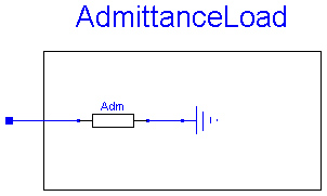
ObjectStab.Loads.AdmittanceLoad

Parameters

Name	Default	Description
P0	1	Rated Load Active Power (at 1 p.u. voltage) [p.u.]
Q0	0.2	Rated Load Reactive Power [p.u.]

Modelica definition

model AdmittanceLoad "Admittance Load" 
  extends Partials.Load;
  ObjectStab.Network.Admittance Adm(G=P0, B=-Q0);
  ObjectStab.Network.Ground Gr;
equation 
  connect(Adm.T2, Gr.T);
  connect(T, Adm.T1);
end AdmittanceLoad;

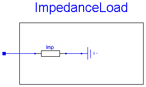
ObjectStab.Loads.ImpedanceLoad

Information

The complex power drawn by the impedance load is:

  Pl+j*Ql = V^2*(R+I*X)/(R^2+X^2)

solving for R and X for given P0 and Q0 yields:

  R = P0*V^2/(P0^2+Q0^2)
  X = Q0*V^2/(P0^2+Q0^2)

Parameters

Name	Default	Description
P0	1	Rated Load Active Power (at 1 p.u. voltage) [p.u.]
Q0	0.2	Rated Load Reactive Power [p.u.]

Modelica definition

model ImpedanceLoad "Impedance Load" 
  extends Partials.Load;
  ObjectStab.Network.Impedance Imp(R=P0/(P0^2 + Q0^2), X=Q0/(P0^2 + Q0^2));
  ObjectStab.Network.Ground Gr;
equation 
  connect(Gr.T, Imp.T2);
  connect(Imp.T1, T);
end ImpedanceLoad;