The aim of this lab is to help you understand:
You should have read chapter 10.1-10.4 in the course book, and you should have a good grasp of heuristic search.
In Part 1 of the lab, you will write your own model of a planning problem and experiment with different planners trying to solve the problem.
The planners you will use all accept the same form of input, a standardized Planning Domain Description Language called PDDL. This language provides a common syntax and semantics for planning formalisms with varying degrees of expressivity. The language is briefly discussed in section 10.1 of the book, and though the book does not use the standard syntax, the concepts discussed are the same as in the book as well as in the lectures.
Here is a short manual on How to write domain and problem definitions in PDDL. This manual also explains some general aspects of PDDL such as its support for STRIPS and ADL expressivity levels. You should read at least that introductory part before you continue reading below.
Many classical planners do not support more features than STRIPS, so if you want to use any ADL features in your own domains and problems, you may have to convert them to STRIPS first by using the adl2strips program, which can be found in ~TDDD17/bin.
There are many approaches to solving planning problems, and many implementations of these approaches.
The planners that we provide in this lab are research prototypes developed by various university research groups. For Part 1, We recommend that in the first place you use the planners LAMA, FF, IPP and VHPOP. They are good representatives of popular approaches, they perform reasonably well and are also quite stable. They also all support some subset of ADL. In particular we strongly recommend you to start with FF as it is a mature implementation and gives rather legible error messages.
LAMA is the winner of the sequential satisficing track of the 2008 International Planning Competition (where "satisficing" means that the plans are not necessarily optimal). One heuristic used is based on a domain analysis phase extracting landmarks, variable assignments that must occur at some point in every solution plan. The landmark heuristic measures the distance to a goal by the number of landmarks that still need to be achieved.
LAMA occasionally gives assertion errors for certain domains and problem instances. If this happens, ignore it and try another planner – this is a bug in the implementation, not in your domain.
FF is a very successful forward-chaining heuristic search planner (see section 10.2 in the course book) producing sequential plans. Although it does not guarantee optimality, it tends to find good solutions very quickly most of the time, and it has been used as the basis of many other planners (such as LAMA). FF does a variation of hill-climbing search using a non-admissible heuristic, which is also derived from plan graphs (like that used by Graphplan, IPP and others).
IPP is a descendant of Graphplan (see section 10.3 in the course book). It produces optimal parallel plans. Graphplan-style planners perform iterative deepening A* search using an admissible heuristic, and use a special graph structure to compute the heuristic and store updates during search.
VHPOP is a partial-order causal-link planner (see section 10.4.4 in the course book). It can work with either ground or partially instantiated actions, and it can use a wide variety of heuristics and flaw selection strategies and different search algorithms (A*, IDA* and hill-climbing). Depending on the heuristic and search algorithm used, the solution may be optimal or not.
In the first part of the lab, you will model a planning domain in PDDL. You can either extend a given domain, or write one from scratch. You should also create at least one problem for your domain, and verify that at least two different planners can solve it.
Feel free to use ADL features (conditional effects, quantified preconditions, etc.) as long as it's supported by at least some planner.
Below are some planning problems for you to choose from. If you want to make up your own problem to model, talk to your lab assistant and/or examiner first to check that it's ok.
If you want, you can make up your own domain to model. If so, please talk to your lab assistant first and verify that your idea is reasonable (not too simple, not too complex).
Here's an example of a rather small world layout:
	-------------------------------------------------------------------------
	|                       |                       |                       |
	|                       |                       |                       |
	|       light switch 1 -|- light switch2        |- light switch3        |
	|                       |                       |                       |
	|       ---             |                     door2                     |
	|       | |           door1      shakey         |                       |
	|       ---           (wide)                    |                       |
	|       box             |                       |                       |
	|                       |                     door3                     |
	|                       |                     (wide)                    |
	|        room1          |        room2          |         room3         |
	-------------------------------------------------------------------------
The following restrictions apply to Shakey's actions:
Shakey can carry small objects, but only two at a time because he has only two grippers.
For Shakey to be able to find a small object in a room, the light must be on in that room.
Shakey can not carry boxes, but can push them around. Boxes can only be pushed through wide doors, not narrow ones.
To switch the light in a room on or off Shakey must climb onto a box that is positioned below the switch (otherwise he can not reach the switch). This may in turn require moving the box into position, possibly from another room.
Typical problems for Shakey may be to find a specific object (e.g. the green block labeled "G") and bring it to a specific place, to turn the lights on/off in every room, or to remove all boxes and objects from one of the rooms (the last problem may require ADL, since the goal is a "for all").
The logistics domain is a standard benchmark in AI planning. In this domain, there are a number of cities and in each city a number of places. The goal is to move a number of packages from their initial places to their respective destinations. Packages can be loaded into (and of course unloaded from) vehicles of different kinds: In the standard domain there are trucks and airplanes. Trucks can only move between places in the same city, while airplanes can only move between places of a certain kind, namely airports.
Here is a definition of the standard Logistics domain, using only the STRIPS subset of PDDL, and a small example problem. The domain and problem definitions are fairly well commented. In the planning/strips directory, there are several more Logistics problems. Files log-3-3.pddl through log-4-4.pddl define increasingly larger problems.
Now you should introduce some complications into the domain:
Introduce some other kind of transportation, e.g. trains, between cities. Like airplanes, trains only "connect" to certain locations within a city. Construct problems in which some cities have only train stations, some have only airports, and some have both.
Make packages of different sizes, and trucks (airplanes, trains, etc.) with different carrying capacity. Note that "counting" is a bit hard to do in the levels of PDDL generally supported by most planners (since there are no numbers), so you'll probably have to settle for classifying packages as "big", "medium" or "small". Note also that there are at least two variations on this theme: For example, you can let e.g. a "small truck" carry any number of "small" packages but no "big" packages, or you can try to formulate a restriction such as "a truck can carry either one big package or three small packages" (the second variant is much more complicated).
In the emergency services logistics domain, a number of persons at known locations have been injured. Your task is to deliver crates containing emergency supplies to each person.
In this lab, we use a comparatively simple version of emergency services logistics:
There are at least three different kinds of crates: food, medicine, and water.
Each injured person is at a distinct location, and either has or does not have a crate of any given type. That is, one person might have a crate of food but lack crates of medicine and water.
The goal specifies which types of crate each person needs. For example, one person might need food and water but not medicine.
Initially all crates are located at a single specific depot location.
Two helicopters are available to deliver crates.
Each helicopter can pick up a single crate, if it is at the same location as the crate. It can then fly to another location with the crate and deliver it directly to a specific person at that location. These are three distinct actions.
Your task is to model this domain in PDDL and construct a couple of problem instances of reasonable size. Solve the problems using several planners and verify that the plans generated are correct.
Hint: Remember that preconditions are generally conjunctive. Saying "there exists no crate that the helicopter is carrying" requires existential quantification, which is disjunctive and can't be handled by many planners. This is instead often commonly modeled by using a predicate "(empty ?uav)" which is set to true in the initial state, made false when you pick up something, and made true when you put something down.
Remember also that goals are generally specified as a single conjunction: (and (something) (somethingelse)). Very few planners handle complex formulas as goals.
After you finish the entire lab including Task 2, you should hand in your domain and problem definition files. The files should be well commented: Explain the way you represent the domain and motivate your choice of predicates, objects and operators.
In the second part of the lab, you will conduct a small empirical investigation of how different general planning heuristics affect a planner based on forward search in the state space.
As a basis for this lab, we will use Fast Downward – a planner that LAMA originated from, and has now been merged back into. The planner is extremely configurable. For example, it can use different state space search methods, heuristics, preferred queues and a lot more. Therefore, this is a planner that can effectively be used to compare different heuristics.
To be able to actually see what the planner does, we have developed our own fork that adds invasive logging. This means that the planner is considerably slower than the original, as every step must be logged into a log file. However, it also means that the planner logs more or less the whole search process, providing the input to our next piece of software, a search space visualizer.
In summary, you will run the planner with different configurations on a given domain and three problems. To measure the performance of the different problems you have to use the visualizer's statistics for heuristic calculations done, states expanded and states visited. (Measuring the search time isn't reliable since the logging increases the time considerably and not by the same amount for every search!) Finally, you will analyse the search procedure for some of them by viewing them in the Graph Visualiser.
The domain that you will use for this task is the nomystery domain. This is a domain from IPC-2011 (international planning competition 2011) that proved hard for many planners in the competition. The domain is essentially a delivery domain where a truck moves between different locations and delivers packages. Moving the truck between two locations consumes fuel which means that the truck can run out of fuel. Make sure that you download the domain and the three problems that you should use.
The first step of the experiment is to run Fast Downward on the three given problem instances and generate a set of logs. If you want to experiment on your own, you can read the general user manual. However, we will provide you with most of the pointers you need here in the lab description.
You run the modified version of Fast Downward as follows, on the IDA lab computers (can also be reached through Thinlinc, but be aware that many others may be using the same terminal servers to run their programs):
$ /home/TDDC17/sw/fdlog/fast-downward.py DOMAIN PROBLEM CONFIGURATION [FLAGS]
The parameters are as follows:
For the experiment you should solve each of the three problems using each of the following three configurations (running Fast Downward nine times):
--heuristic 'hff=ff()' --search 'eager_greedy([hff])'
This configuration combines eager greedy search (greedy = always select the expanded-but-not-visited node with the lowest heuristic value in the queue, eager = when you create a new state, immediately compute its heuristic value) with the heuristic function used by the FF (FastForward) planner.
--heuristic 'gc=goalcount()' --search 'eager_greedy([gc])'
This configuration still uses eager greedy search, but the heuristic function is based on how many of the goals remain unsatisfied. In other words, always pick from the queue one of the expanded-but-not-visited nodes with the minimum number of facts left to achieve. As we discussed during the lectures, this heuristic seems intuitive but does not provide particularly good guidance.
--heuristic 'gc=goalcount()' --heuristic 'hff=ff()' --search 'eager_greedy([gc], preferred=[hff], boost=x)'
Where x is the number of items that should be taken from the preferred queue (see below).
In addition to ordinary heuristics, many successful planners also use other "tricks" to distinguish between useful and less useful paths through the search space.
One such trick is the computation of helpful actions. A simple and mostly accurate explanation would be that in each state, the planner very quickly solves a simplified variation of the problem, where certain action conditions that complicate the search process are completely ignored. Since some conditions are ignored, this only generates a "pseudo-solution" that cannot be used as the actual output of the planner. However, some important conditions have still been checked, so many completely irrelevant actions have been ruled out, and the actions in the "pseudo-solution" are more likely to be useful in the real problem on average.
How can this "probability of usefulness" actually be used? By using two queues of actions to be tested, one that only contains helpful actions (which ensures these are tested more often), and one that contains all actions that were not identified as helpful (because like any heuristic, the computation is not perfect and can miss actions that are not only helpful but even necessary). In essense, as soon as a search node that has a lower heuristic value according to the FF heuristic is visited, x items will be taken from the queue consisting of all the expanded but not visited nodes that was reached by using a preferred operator (according to the FF heuristic).
In our example below, helpful actions are used to decide which queue an action ends up in, while the goal count heuristic is used to order the items within each queue.
A good value for x on the problem instance that you are going to use is 256.
We can get some insights into what the planner is doing from looking at the statistics that are generated for each search. These statistics include the following interesting numbers (which has a slightly different terminology than what you are most likely used to):
However, we can see far more if we use the graph visualizer.
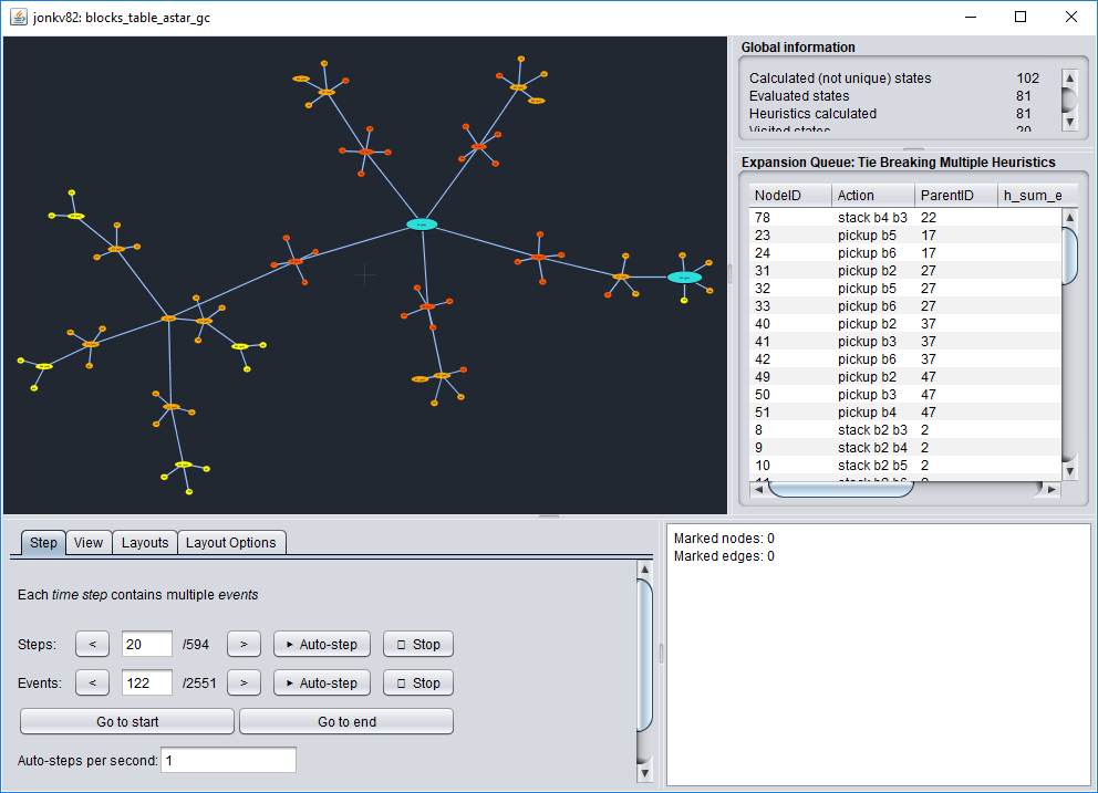
The Graph Visualiser is a tool that is written at IDA that is used to debug planners and other graph based algorithms. It can display graphs and more importantly go through a search log file step by step.
The Graph Visualiser requires that you run java version 1.8. This isn't the default java version on the linux machines. Therefore, you have to run it using the following:
/sw/jdk1.8.0_45/bin/java -jar /home/TDDC17/sw/fdvis/fdvis.jar path/to/log-file
Where path/to/log-file is the path to the log file that Fast
Downward produced. This file should be produced in the same folder
as you executed the script in and is named stats.txt
(or stats.gz
if you used the
--compressflag).
You should now look at what the planner actually did for some of the configurations you tested!
First, make sure you play around with the visualizer. Choose an arbitrary log file among those that you generated, start the visualizer, step forward and back, and test the different options for Node coloring in the View pane. For example, "Colour Map[g]" lets you color nodes by their g value (the cost of reaching a node), while "Colour Map[h_goal_count]" refers to the goal count heuristic (red = high, green = low). More information is shown in the manual!
Then answer the following questions based on running the visualizer on the problems specified below (don't forget screenshots):
Start the Fast Downward visualizer twice, using the log files generated when solving problem 03 with the configuration that uses (a) FF-heuristic and (b) goal count heuristics, respectively.
Step both visualisations to time step 40 manually or through auto-stepping. Don't use the "go to" functionality (entering a step number) because you will need to see nodes as they appear!
How do the graphs differ, given the same problem and search method but different heuristics? Include screenshots in your report and discuss what you see!
Again step both visualisations to time step 40 manually or through auto-stepping. Don't use the "go to" functionality.
How many dead ends have the two searches encountered? Include screenshots of the graphs!
Do the different configurations use different actions? Zoom in on the edges to see which actions are used and discuss the differences.
Step the FF visualisations to the end through
auto-stepping (hint: set the Auto-steps per second
to a value higher than one but small enough so that you
can follow the search process). Don't use the go to
functionality.
Was the original expanded path used in the final plan?
Run the Fast Downward visualisation on the log files generated when solving problem 02 with the configuration that uses FF-heuristic and the one using GC heuristics with preferred operators from FF.
When the planner adds a new action to a branch in the search tree, this doesn't necessarily cause the heuristic function to decrease. In which time step does the planner first find a new lower value for the main heuristic function in each example (FF and GC, respectively)?
Step both visualisation to time step 27 (the last time step with the configuration using FF as heuristic).
How many goals left to solve according to the goal count heuristic in the state that has progressed the longest?
Auto-step the visualisation for the goal count heuristic to the end.
Follow the marked path from the start node to the first goal node that is found. Does the solution ever increase the value of the goal count heuristic between one state and the next?
Run one of the configurations on your own domain and problem. Is the graph similar to any of those that you have examined above? Can you explain why or why not?
You should hand in a report describing you findings in this experiment. This should include (but don't hesitate to add more if you had findings outside the questions here):
Questions/answers may be added during the course.