Alignment Cubes:
Towards Interactive Visual Exploration
and
Evaluation of Multiple Ontology Alignments
Valentina Ivanova1, Benjamin Bach2, Emmanuel Pietriga3, and Patrick Lambrix1
1 Swedish e-Science Research Centre and Linköping University, Sweden
2 University of Edinburgh, United Kingdom
3 INRIA, LRI (Univ Paris-Sud & CNRS), Université Paris-Saclay, France
Ivanova V, Bach B, Pietriga E, Lambrix P, Alignment Cubes: Towards Interactive Visual Exploration and Evaluation of Multiple Ontology Alignments, 16th International Semantic Web Conference, LNCS 10587, 400-417, Vienna, Austria, 2017.
Introduction
The quality of ontology alignments is often evaluated by comparing them against reference alignments and computing measures, such as precision, recall and F-measure. These measures, however, provide only an overall assessment of alignments' quality; they do not allow for comparing alignments of specific parts of ontologies, or for comparing alignments to each other and to the reference alignment at the detailed level of concepts and relations. In many cases reference alignments are not available which makes comparison of alignments at different level of detail even more important.
AlignmentCubes is a tool which allows for interactive visual exploration of several ontology alignments and thus supports alignments' evaluation at different levels of detail. These are some use cases in which AlignmentCubes will be very helpful:
- Selecting, combining and fine tuning alignment algorithms and tools;
- Matchers development;
- Ontology alignment evolution;
- Validating and debugging of ontology alignments and reference alignments;
- Collaborative ontology alignment.
Tool & Datasets
Running the tool and example data
You can find below a runnable jar with the tool (run by using the command below or double click on the file).
java -jar AlignmentCubes.jar
Each dataset contains both ontologies, a folder with alignments and a file with performance measures.
Notes:
- The first ontology is loaded on the green axis, the second on the red axis, and the alignments (max. 15) on the blue axis.
- The initial loading takes some time due to the number of libraries.
Tool: AlignmentCubes_v_0_1.jar (java 8), User Manual
Example Datasets: Datasets.zip
Figures from the submission
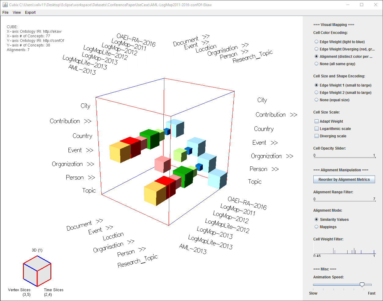
Fig 2: Alignment Cube UI. Widgets (sliders, button groups, etc.) mentioned in the text are referred to directly using their name. The cubelet (bottom left corner) is used to switch between views by clicking or dragging the mouse on its faces.
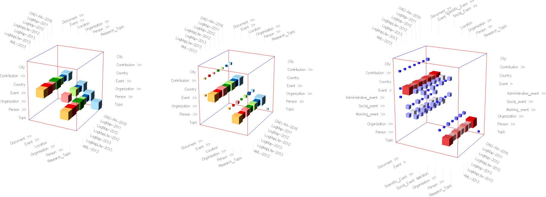
Fig. 3: Alignment Cubes for visualizing ontology alignments. Rows and columns of the cube represent ontology concepts, individual cells inside the cube represent mapping relationships. Each alignment, corresponding to a slice in the third dimension, is assigned a different color. (a) Default view in similarity values mode. (b) Initial view in mappings mode. (c) Mappings mode with cell weight color encoding after expanding the Events concepts in both ontologies.
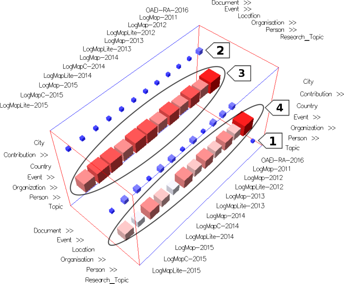
Fig. 4-A: 3D view in mappings mode: initial view.
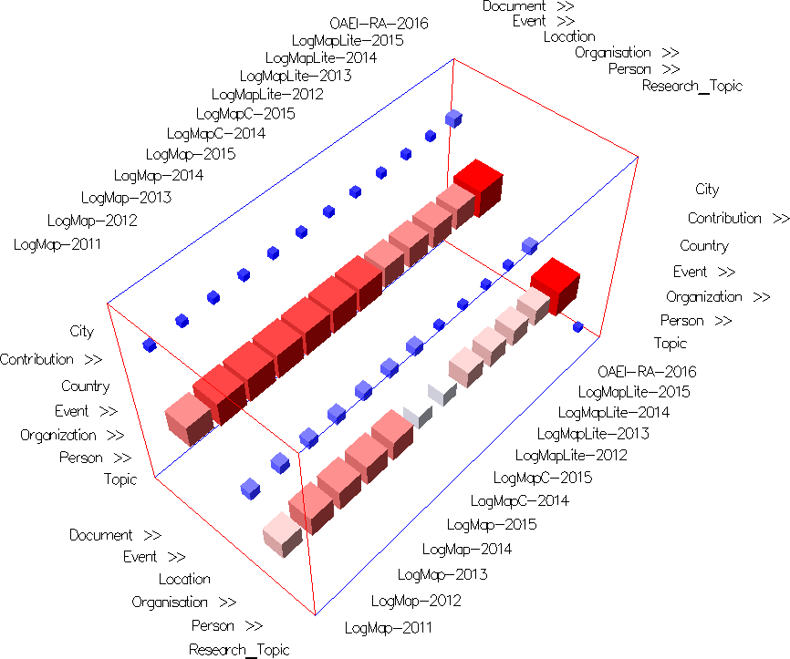
Fig. 4-B: 3D view in mappings mode: after reordering by name.
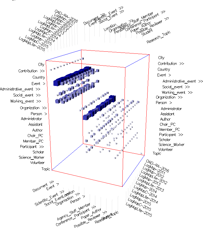
Fig. 5-A: Views of Alignment Cubes: after expanding concepts.
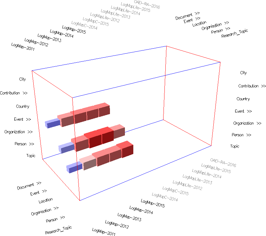
Fig. 5-B: Views of Alignment Cubes: after filtering out several alignments.
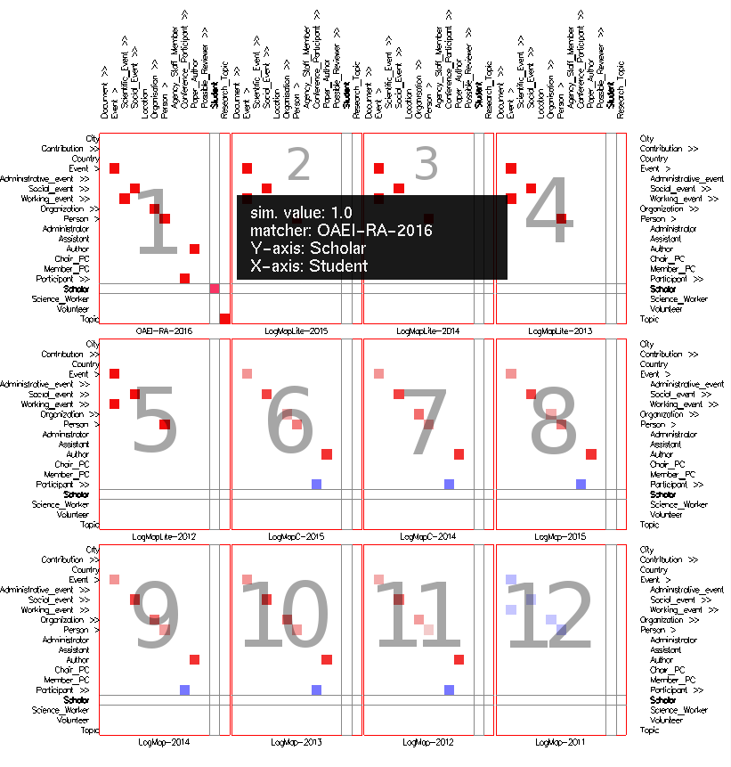
Fig. 6-A: Small-multiples views: alignment topology. Gray numbers have been added manually to the figure.
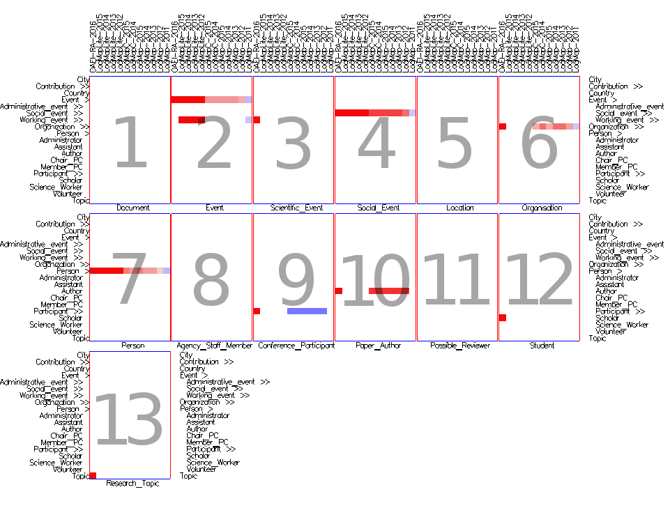
Fig. 6-B: Small-multiples views: concept networks. Gray numbers have been added manually to the figure.
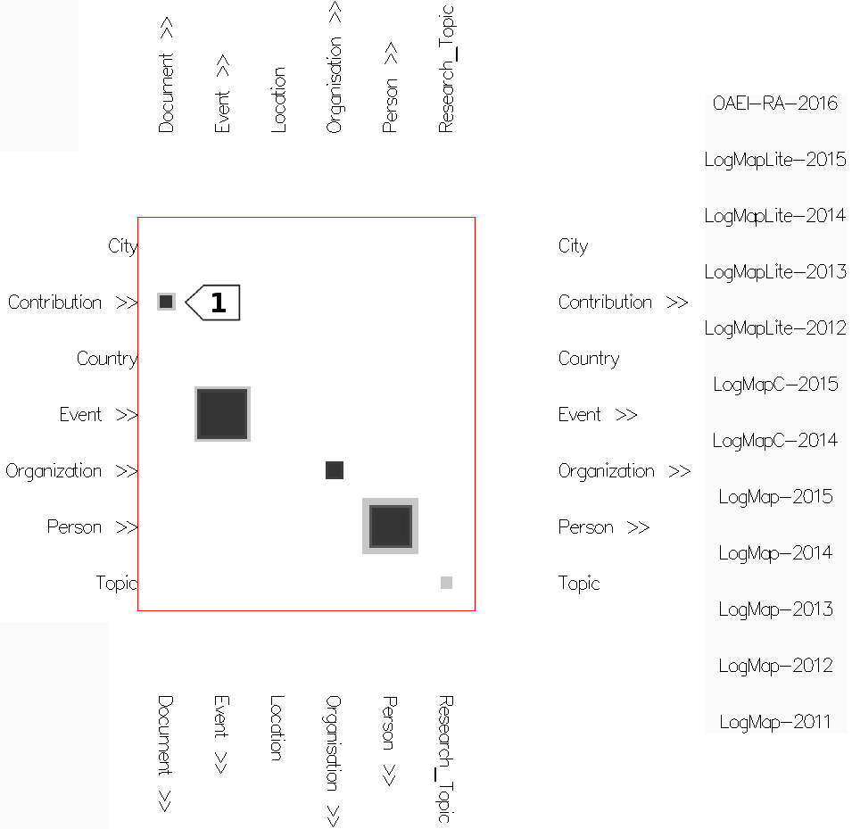
Fig. 7-A: Aggregated projections: alignment topology.

Fig. 7-B: Aggregated projections: concept networks.
User Manual
Alignment Cubes Interface
The Alignment Cubes interface in its initial 3D cube view is presented in Figure 1.
The color of the axis is permanently mapped to one of the cube's dimensions as follows:
- The red axis shows the source ontology (loaded first in the file chooser).
- The green axis shows the target ontology (loaded second in the file chooser).
- The blue axis shows the alignments which are computed by the different matchers or systems (the path to the folder with alignments in ALlignment API format is loaded in the third field in the file chooser).
Initially, only the first level of concepts (concepts directly under owl:Thing) from both ontologies are shown. The taxonomic hierarchy of the ontologies is presented as collapsible indented lists. Concepts that feature sub-concepts display the >> symbol after the concept label (e.g., Event, present in both ontologies, features sub-concepts). Clicking on a concept label expands the corresponding row or column. Expanded concepts then show the > symbol, and sub-concepts are indented according to their level in the hierarchy. Concepts that have multiple parents appear under each parent, i.e., potentially multiple times in the hierarchy.
Alignments Modes:
Alignment Cubes features two alignment modes in order to accommodate views at different levels of granularity:
- In similarities mode, a filled cell represents an existing mapping between a pair of concepts. The cell's weight represents the similarity value. This mode allows to compare the similarity values computed by the different matchers or systems.
- In mappings mode, a filled cell indicates that there is at least one existing mapping between a pair of concepts or their descendants; the cell's weight represents the number of mappings. This mode allows to identify parts of the alignments with few or many mappings. When a concept is expanded, in this mode, a cell is shown for both the concept itself and its sub-concepts. This forms regions in the cube where smaller cells indicate mappings deeper in the hierarchy.
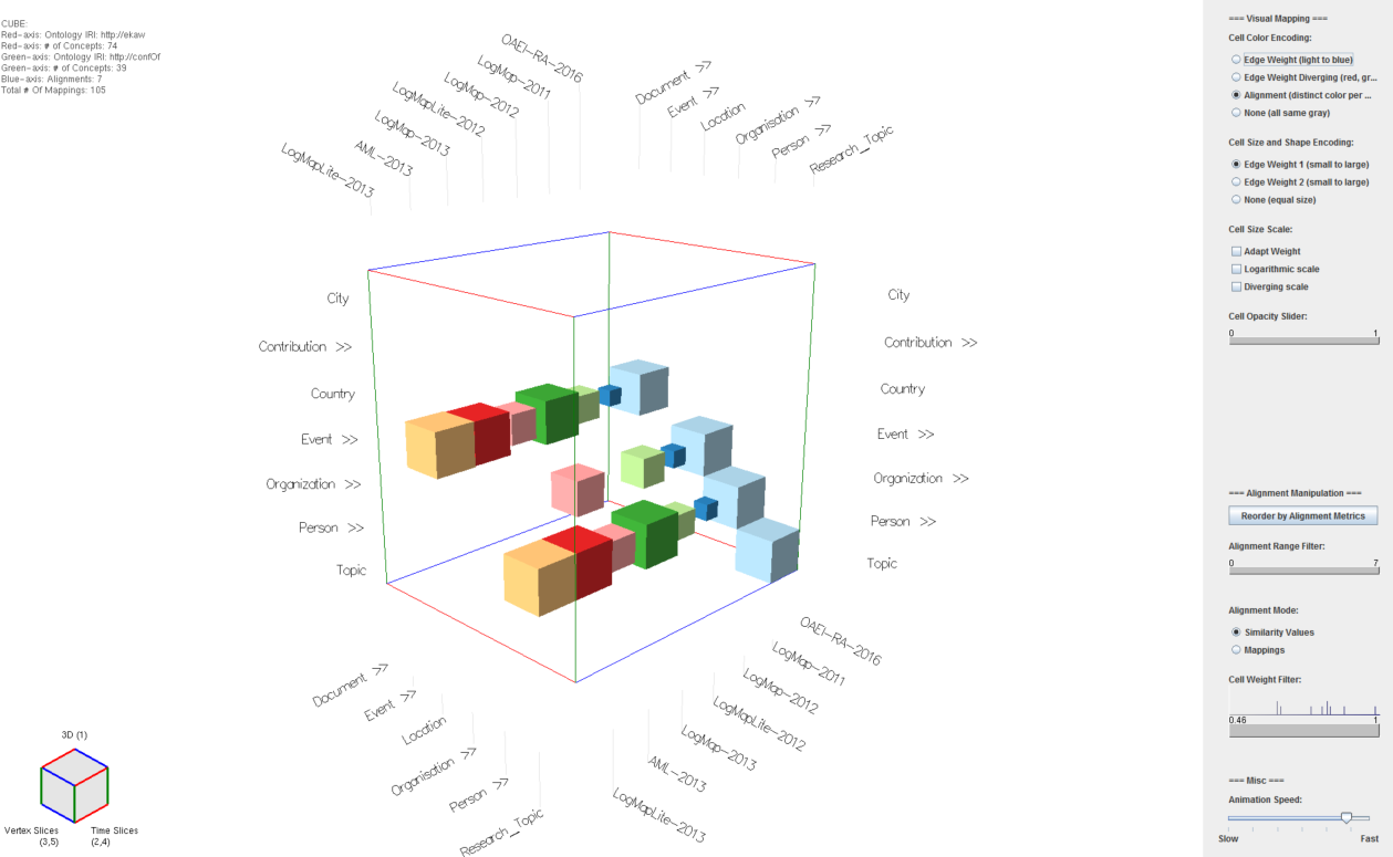
Fig. 1: Alignment Cubes UI. Widgets (sliders, button groups, etc.) mentioned in the text are referred to directly using their name.
Views:
- 3D cube view - initial view - Figure 1. The cubes that belong to one alignment are colored in the same color (using Alignment Color Encoding option), e.g., the yellow cubes belong to the alignment generated by LogMapLite-2013.
- Projection views - aggregated views:
- In the alignment topology projection view (Figure 2) all alignment matrices are overlaid on top of each other. The columns of the resulting matrix hold the concepts from the source ontology, the rows hold the concepts from the target ontology. The alignments are presented on the right side of the matrix, hovering on them shows the respective matrix. This view provides an overview of the aggregated mappings for each pair of concepts between both ontologies.
- In the concept network projection view (Figure 3) all matrices for a concept from the source ontology are overlaid on top of each other. The columns of the resulting matrix hold the matchers, the rows hold the concepts from the target ontology. The concepts from the source ontology are presented on the right side of the matrix, hovering on each shows the respective matrix. This view provides an overview of the mappings computed by the different matchers or systems.
- Small multiples views - detailed views:
- In the alignment topology small multiples view (Figure 4) all alignments are spread and juxtaposed next to each other, i.e., there is one matrix per alignment where the columns and rows come from the source and target ontologies respectively. Thus this view provides a detailed view of each alignment.
- In the concept network small multiples view (Figure 5) the matrices for the visible concepts in the source ontology are spread and juxtaposed next to each other, i.e., there is one matrix per concept from the source ontology. Thus this view provides a detailed view of all mappings for a concept from the source ontology.
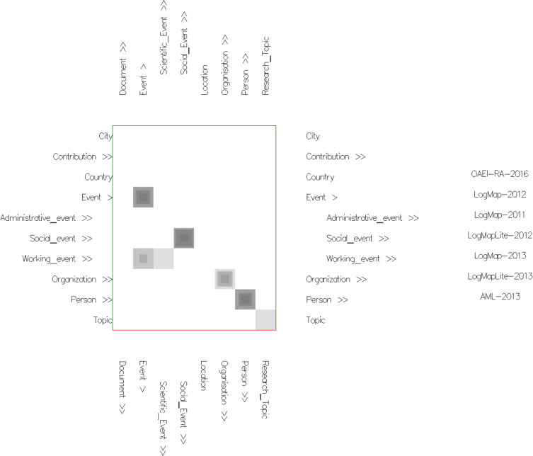
Fig. 2: Alignment topology projection view in similarities mode with uniform cells' color (using None Color Encoding) and semi-transparent cells (using Cell Opacity Slider). Nested cells indicate different similarity values (disagreement between matchers). Darker and non-nested cells indicate higher agreement between matchers.
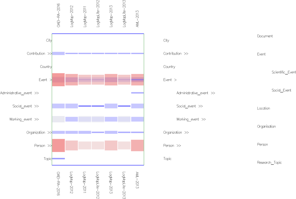
Fig. 3: Concept network projection view in mappings mode with cells colored according to their weight (using Edge Weight Diverging Color Encoding), stretched cells (using Edge Weight 2 Shape Encoding) and semi-transparent cells (using Cell Opacity Slider). Nested cells indicate existing mappings between different regions in the ontologies (including sub-regions in case of expanded concepts). For instance, the nested cells on the Event row indicate there are mappings between confOf:Event (in the matrix) or its descendants and concepts from the ekaw ontology on the right of the matrix. Hovering on the ekaw concepts (the indented list) we see that most of the mappings are between confOf:Event and ekaw:Event, ekaw:Scientific_Event, ekaw:Social_Event and in one case between confOf:Event and ekaw:Document.
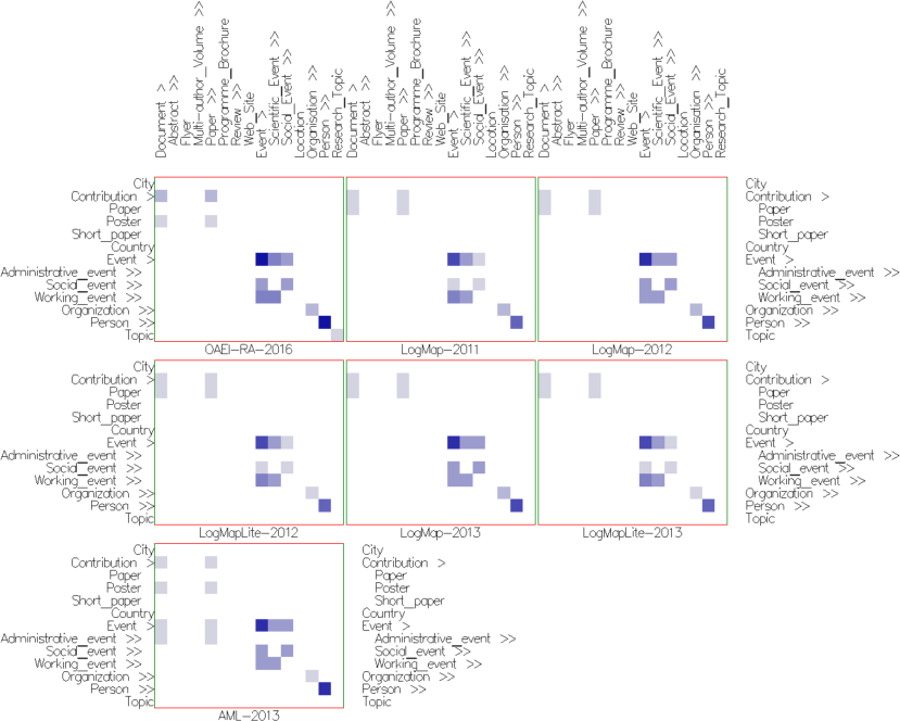
Fig. 4: Alignment topology small multiples view in mappings mode with cells colored according to their weight (using Edge Weight Color Encoding), and uniform size (using None Size Encoding). These settings allow to visually compare parts of the alignments computed by the different matchers. The cells in the intersection of both Event concepts and their descendants indicate that there are mappings in this part in all alignments. The lighter cells indicate under which sub-concepts the single mappings are located. Observing cells' color in the same part shows similar behavior in LogMap-2012 and LogMap-2013 on one side and LogMap-2011, LogMapLite-2012 and LogMapLite-2013 on another. On the contrary, the same cells' number and color around the Contribution row in all LogMap-family systems indicate same matchers' behavior for this part in all alignments.
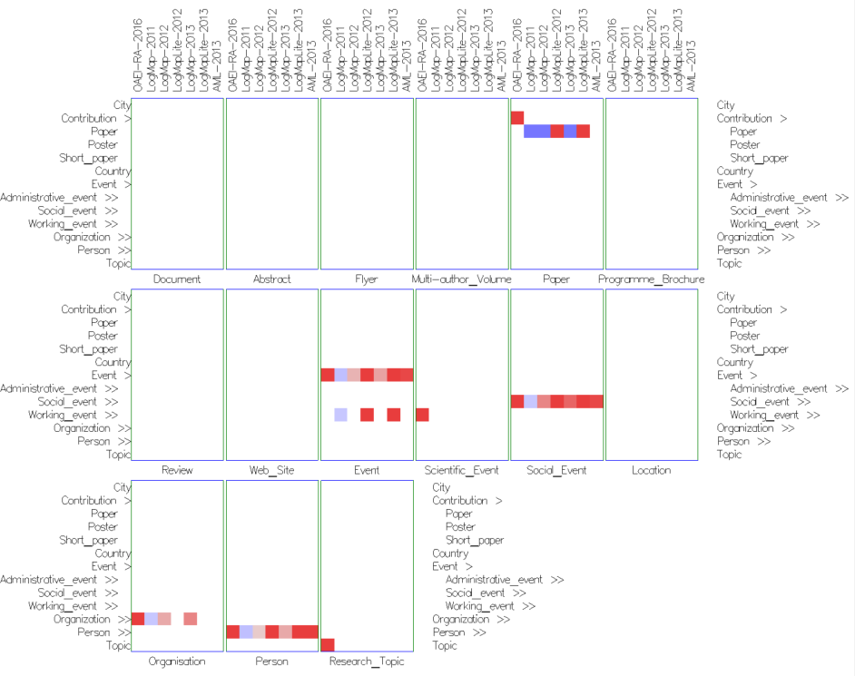
Fig. 5: Concept network small multiples view in similarities mode with cells colored according to their weight (using Edge Weight Diverging Color Encoding), and uniform size (using None Size Encoding). There is one matrix for each visible concept form the ekaw ontology. The single cell in the ekaw:Research_Topic matrix indicates that the mapping has been found only in the reference alignment, but not by other matchers. Similarly, in the ekaw:Paper matrix the single cell in the confOf:Contribution row indicates that the mapping has been found only in the reference alignment. In the same matrix, most of the matchers have found a wrong mapping between confOf:Paper and ekaw:Paper.
Navigation Between the Views:
Switching between the views is performed by clicking or dragging the mouse on the faces of the cubelet widget (bottom left corner on Figure 1).
- 3D cube view is accessed by clicking on the top cubelet's face.
- Projection views:
- Alignment topology view is accessed by clicking on the right cubelet's face.
- Concept network view is accessed by clicking on the left cubelet's face.
- Small multiples views:
- Alignment topology small multiples view is accessed by dragging the right cubelet's face.
- Concept network small multiples view is accessed by dragging the left cubelet's face.
Further Visual Exploration Features:
Multiple widgets provide a variety of interaction to support interactive visual exploration of the alignments.
Visual Mapping:- Cell Color Encoding:
- In Edge Weight (light to blue), cells are colored according to their weight, ranging from light blue (low weight) to dark blue (high weight). This encoding helps heavy edges, i.e., cells with higher weight, to stick out as dark cells.
- In Edge Weight Diverging (red, gray, blue), cells are colored according to their weight, ranging from blue (lowest values) to red (highest values). With this encoding cells with high and low weights are contrasted.
- In Alignment (distinct color per matcher), cells are colored according to the matcher that has calculated them. This encoding helps identifying all mappings belonging to one alignment. This is the default color encoding.
- In None (all same gray), cells are colored in the same dark gray. When applying opacity to cells and seeing the cube in a projection view, more cells overlapping on top of each other will result in darker cells thus denoting existing mappings for pairs of concepts presented in many alignments.
- Cell Size and Shape Encoding:
- In Edge Weight 1 (small to large), cell size indicates weight in a linear scale. Larger cells indicate higher weight, smaller cells indicate lower weight. The cell weight represents either the similarity value (in similarities mode), or the number of mappings (in mappings mode). This is the default size and shape encoding.
- In Edge Weight 2 (small to large), instead of cubes, cells are ”stretched” to connect with the other cells, i.e., mappings, for a pair of concepts. This results in visually connecting together all mappings for a pair.
- In None (equal size), all cells have equal size. This is useful to i) get a better impression of mappings density (number of cells in the cube, i.e., mappings in the alignments), and ii) when cells get very small in the small multiples views.
- Cell Size Scale:
- In Adapt Weight, cell size is rescaled according to the weight of the visible cells. The cell with the lowest edge weight that is visible is mapped to the smallest size, while the cell with the highest weight that is visible becomes largest.
- In Logarithmic scale, cell weight is mapped in a logarithmic way to cell size. This encoding is helpful when there are cells with large differences in the weight.
- In Diverging scale, cell size is rescaled using a scale between 0 and the maximum weight value of the visible cells.
- Cell Opacity Slider - changes the transparency of the cells thus allowing for seeing through them. The right handle of the slider sets the opacity of the visible cells. The left handle of the slider sets the opacity of filtered out cells, i.e., either not in the current range of alignments or not in currently selected slices. This allows to explore the cube, while not completely removing all filtered out cells.
- Alignment Range Filter - allows to see only some of the alignments by filtering out those alignments at the beginning (when using the left handle) or at the end (when using the right handle) depending on their ordering.
- Cell Weight Filter - filters out cells above (when using the right handle) or below (when using the left handle) a particular edge weight range. A histogram above the slider indicates the distribution of edge weights across the scale. When the Adapt Weight size scaling is active, the remaining cubes are scaled so that their size varies according to the currently visible weight range. This means that cells at the lower range of visible weight are very small, while cells on the higher end have maximal size. Such an adapted weight range allows to better perceive the weight distribution within a given weight range.
- Concept/s - slices for particular concepts can be selected by clicking on the corresponding labels. Non-selected slices are either invisible or rendered translucent depending on the value set by the left handle of the Cell Opacity Slider.
- Reorder by Alignment Metrics - changes the order of the alignments considering measures such as precision, recall and F-measure. The alignments can also be reordered alphabetically by the alignments' (matchers', systems') names. Ordering remains consistent across views.
- Slice Coloring - Slices can be colored manually to track their cells across views by pressing Shift and click on the desired slice label. Another click removes the coloring. Colors are assigned randomly.
Controls:
Keyboard Controls:- Key 1 - 3D cube view
- Key 2 - Alignment topology projection view
- Key 3 - Concept network projection view
- Key 4 - Alignment topology small multiples view
- Key 5 - Concept network small multiples view
- Drag mouse + left button - rotate cube
- Drag mouse + right button - pan
- Scroll mouse wheel - zoom
- Shift + click on slice label - color slice (do the same to return the slice color to its initial value)
- Alt + scroll mouse wheel - change labels size
Under Development:
Additional Views:- Context views to observe individual slices when in one of the aggregated projection views:
- Alignment topology context view (Figure 6) is accessed by a right click on a column label in the alignment topology projection (another click closes it).
- Concept network context view is accessed by a right click on a column label in the concept network projection (another click closes it).
- Another pair of concept network views with the same functionality as the current pair but for the concepts in the target ontology
- Investigating alternatives to visually represent different types of mappings (subsumption, equivalence, asserted, derived, etc.);
- Visualizing the results of set operations (union, intersection, complement) between alignments;
- Exploring clustering and reordering algorithms to further support trends and patterns discovery.
- Implemented: Loading the alignments directly from the alignment files without preprocessing to merge all of them into one file.
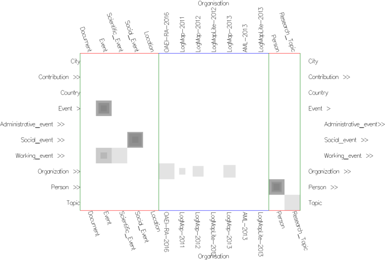
Fig. 6: Alignment topology context view in similarities mode with uniform cells' color (using None Color Encoding) and semi-transparent cells (using Cell Opacity Slider). While exploring the alignment topology projection view in Figure 2, we have noticed the nested cells in the intersection of both Organization concepts. A right click on the Organization column opens the respective slice and allows to inspect the values for the pair computed by the different matchers.