Chapter

This chapter provides a brief introduction to LiUPTS program.

iUPTS is a tool set developed at Embedded Systems Lab (ESLAB), Linköping University to help the study of P1687 networks. LiUPTS mainly contains the implementation of two sets of algorithms, i.e. IJTAGcalc [1] and PACT [2]. The IJTAGcalc set of algorithms calculate the test application time (TAT) for a given IEEE P1687 (IJTAG) network, and for the concurrent and sequential schedule types. The PACT (P1687) set contains algorithms to construct P1687 networks optimized with respect to TAT, and for concurrent and sequential schedule types. LiUPTS code is written in C++ .NET using Microsoft Visual Studio 2008 Express Edition [3]. The source code might also be made available upon request. This user’s guide will describe how IJTAG networks are described, as taken as input and generated as output by LiUPTS, and how this tool set can be used to construct and analyze P1687 networks. It is assumed that the user is familiar with IJTAG terms such as Gateway, SIB, HIP and etc. Otherwise he/she is encouraged to take a look at the Appendix A for a list of resources which describe these terms. Of course since the final draft of the P1687 standard is not yet out at the time of preparation of this manaul, the terminology in this area is not quite established and is prone to changes.

The rest of this document is organized as follows:

· Chapter 2 will describe how an IJTAG network is described as required (and is generated) by LiUPTS.

· Chapter 3 will describe the Graphical User Interface of LiUPTS.

Chapter

Representation of IJTAG Networks

This chapter discusses how IJTAG networks are described, using Extensible Markup Language (XML) to be used by LiUPTS.

ML provides a standard way of representing information and it is handy when it comes to describing hierarchical structures. Therefore, XML is chosen (instead of plain text) by LiUPTS developers for describing IJTAG networks (which are hierarchical by design). In this chapter we will start by describing building blocks of IJTAG logic using XML and will conclude with an example which makes use of these building blocks.

Important Note

The use of XML, and the way that it is used, to describe IJTAG networks is merely the choice of LiUPTS developers. That is, this idea is NOT at all related with the decisions of the P1687 working group [4].

Empty Design Skeleton

Listing 1 shows the minimum XML code required to describe an IJTAG network:

Listing 1

1: <?xml version="1.0"?>

2: <Gateway SCLength="0" SCPatterns="0">

3: </Gateway>

The first line simply states that this is an XML document. This line will only be used once in every XML document. Line 2 and Line 3 together define the Gateway which is the interface of IJTAG network to the JTAG TAP. The SCLength=”0” and SCPatterns=”0” are called attribute/value pairs, which will be explained thoroughly when describing Segment Insertion Bit (SIB). These attribute/value pairs will be used in case an instrument is directly connected to the Gateway in series with other SIBs. A value of zero assigned to SCLength and SCPatterns means that no instrument is directly connected to the Gateway.

Note

Please notice that XML documents are case sensitive and neglecting this will lead to run-time errors!

Segment Insertion Bit (SIB)

SIBs are used to either connect an instrument to the IJTAG circuitry or act as a doorway to another layer of hierarchy. So, in order to differentiate these two types of SIBs in this manual, they are called instrument SIBs and doorway SIBs respectively. But for describing both types the same XML tag which is <SIB></SIB> will be used. The following shows how an instrument SIB is described along with its associated instrument:

The “/>” token is the shorthand for writing “></SIB>” in XML. So the above can also be written as:

Here, SCLength states the length of the internal shift-register associated with the instrument, and SCPatterns states the number of times that the instrument is to be accessed. The ID attribute is currently ignored by the tool but it can be used by the user to differentiate the SIBs in a large file.

NOTE

Any attribute/value pair not discussed in the manual is ignored by LiUPTS and no error is raised!

Figure 1 shows the conceptual schematic of the SIB described above. L denotes the length of the shift-register inside the instrument and P denotes the number of times the instrument is to be accessed. TDI and TDO stand for Test Data Input and Test Data Output respectively.

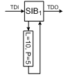
Figure 1 shows a conceptual view of an instrument SIB and its associated instrument.

Please notice that the XML shown above for Figure 1, should be placed inside the “<Gateway>” and “</Gateway>” tags (in the XML shown in Listing 1) to be usable by LiUPTS. So the complete XML description of the structure in Figure 1 will be as shown in Listing 2.

Listing 2

1: <?xml version="1.0"?>

2: <Gateway SCLength="0" SCPatterns="0">

3: <SIB ID="1" SCLength="10" SCPatterns="5"/>

4: </Gateway>

In Listing 2, SCLength=”10” and SCPatterns=”5” correspond to L=10 and P=5 in Figure 1, respectively.

To describe a doorway SIB, the SCLength and SCPatterns attributes are set to zero and the segment of the P1687 network connected to the HIP of this doorway SIB is described between the starting and ending tags- i.e. between “<SIB>” and “</SIB>”. For example, if two instruments similar to what is shown in Figure 1 are to be connected to the HIP of a doorway SIB- as shown in Figure 2, the XML shown in Listing 3 should be used. In this manual, SIB₂ and SIB₃ are referred to as children of SIB₁.

Listing 3

1: <SIB ID="1" SCLength="0" SCPatterns="0"/>

2: <SIB ID="2" SCLength="10" SCPatterns="5"/>

3: <SIB ID="3" SCLength="10" SCPatterns="5"/>

4: </SIB>

Using the same tag for both types of SIBs also allows us to describe a SIB whose HIP is used to both connect to an instrument and to one or more SIBs. The XML shown in Listing 4 describes the schematic shown in Figure 3.

Listing 4

1: <SIB ID="1" SCLength="20" SCPatterns="4"/>

2: <SIB ID="2" SCLength="10" SCPatterns="5"/>

3: </SIB>

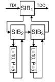
Figure 2 shows a doorway SIB with two instrument SIBs on its HIP

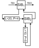
Figure 3 shows a SIB having both an instrument and another SIB on its HIP

Table 1 summarizes the above discussion on the significance of SCLength and SCPatterns values. In Table 1, the two bottom rows show that any negative value for these attributes will NOT raise an error, and therefore care must be taken to avoid undetectable mistakes!

Table 1 discusses the significance of the combination of SCLength and SCPatterns attributes of a SIB tag.

SCLength	SCPatterns	Has children?	Comments
		No	The SIB will be considered as an instrument SIB. If SCPatterns=0, it is assumed that the output of the instrument is to be read only once, without applying any inputs.
	Any value	No	The SIB will still be considered as an instrument SIB with a loopback on its HIP! It is opened once (which takes a CUC) and represents a delay on the scan-path.
	Any Value	Yes	The SIB will be considered as a doorway SIB.
		Yes	The SIB will be considered as a doorway SIB having an instrument on its HIP in series with its child SIBs, see Figure 3. If SCPatterns=0, it is assumed that the output of the instrument is to be read only once, without applying any inputs.
	Any Value	Any Value	Wrong results will be generated without raising any errors!
Any Value		Any Value	Wrong results will be generated without raising any errors!

Dealing with IEEE 1500 Standard Wrapped Instruments

This initial release of LiUPTS can only handle the so called “Localized Control” way of handling wrapped cores [4]. Briefly put, in the “Localized Control” method the SIB contains an additional pair of Capture/Update registers to control the SelectWIR input of the 1500 wrapper serial port (WSP). This extra pair of registers implies an additional delay through the SIB. To access the scan-chain inside the wrapped core, first the Wrapper Instruction Register (WIR) should be selected which should be done at the same time that the SIB is opened. Then the instruction required to activate the desired scan-chain should be shifted in the WIR of the wrapper. After a Capture/Update Cycle (CUC) the instruction is updated and decoded, and the scan-chain is activated and ready to receive input. To describe a wrapped instrument and its associated SIB, it suffices to add a WIRLength attribute along with its value to the “<SIB>” tag. WIRLength attribute specifies the length of the WIR. Upon encountering the WIRLength attribute in the input file, LiUPTS treats the logic described by the SIB as a wrapped core. That is, first data should be shifted in the WIR and after a CUC the rest of the logic described by that SIB is taken into account.

NOTE

If WIRLength attribute has a value smaller than one, it is ignored.

Figure 4 shows a conceptual schematic of a 1500 wrapped core along with its SIB. In this Figure, the box containing the letters “WIR” represents the Wrapper Instruction Register and L specifies the length of that register. Also, the box containing SC represents the scan-chain contained in the wrapped instrument where L specifies the length of the scan-chain and P specifies the number of stimuli that are to be applied. The box next to SIB₁ represents the extra pair of registers that are required to control the SelectWIR input of WSP. It is shown as a box separate from the SIB itself to emphasize one additional delay on the TDI -TDO path. LiUPTS assumes that this extra pair of registers is placed before the SIB on the scan-path. It should be noted that this assumption has an impact on the test time calculations when the pipelining registers (as will be introduced in the following chapter) are assumed to be in use.

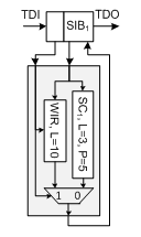
Figure 4 shows a conceptual view of a wrapped scan-chain as well as its associated SIB

The XML description of the structure shown in Figure 4 is:

Or simply:

If instead of a scan-chain a more complex logic is wrapped, such as an IJTAG network, it can be described by placing its XML description between “<SIB>” and “</SIB>” tags.

An Example

Figure 5 shows an example IJTAG network which can be described by the XML document shown in Listing 5.

Listing 5

1: <?xml version="1.0"?>

2:

3: <Gateway SCLength="0" SCPatterns="0">

4: <SIB ID="1" SCLength="20" SCPatterns="4" WIRLength="10">

5: <SIB ID="3" SCLength="8" SCPatterns="2"/>

6: </SIB>

7: <SIB ID="2" SCLength="10" SCPatterns="5"/>

8: </Gateway>

Here, line 2 shows how XML comments look like. The rest is described is previous sections.

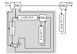
Figure 5 shows a rather complex logic described by Listing 5. The shaded area marks the wrapped logic.

Chapter

Graphical User Interface

In this chapter, the features of LiUPTS will be introduced and using those features through the Graphical User Interface (GUI) will be discussed.

LiUPTS provides the following main features:

· Calculation of test application time (TAT) for a given P1687 network using two schedule types: concurrent schedule and sequential schedule. TAT calculation is based on the algorithms proposed as IJTAGcalc in [1].

· Construction of P1687 networks (given a set of instruments, and for the concurrent and sequential schedule types) which are optimized with respect to TAT for the given schedule type. Network construction is based on the algorithms proposed as PACT in [2].

In addition, LiUPTS provides the following utilities:

· Construction of P1687 networks (given a set of instruments) having flat architecture or regular hierarchical architectures such as binary trees, ternary trees and etc.

· Generation of a list of scan-chains with random number of patterns and lengths.

We will continue this chapter by describing each of these features.

Test Application Time (TAT) Calculation

The current version of LiUPTS supports two test schedule types- namely concurrent and sequential schedules, and reports detailed information such as different types of overhead. To use the TAT calculation feature, select the “Analyze Design” tab and push the “Browse for Design” button to select the design file. After selecting the file, the name of the selected design file appears in the status bar and the “Select calculation method” drop-down menu and the “Calculate” button become enabled, as shown in Figure 6. After selecting the TAT calculation method from the drop-down menu and pushing the Calculate button, the result is shown in the “View Report” tab- as shown in Figure 7.

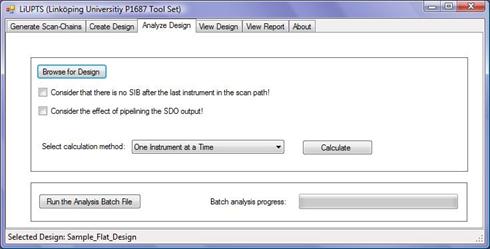
Figure 6 shows the analysis feature of LiUPTS

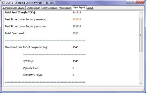
Figure 7 shows a sample TAT calculation report

In the report, “Test Time Lower Bound (Theoretical)” and “Test time Lower Bound (Calculated)” show the shifted test data where the former is calculated based on the instruments list and the latter is calculated during the TAT computation. These two should always show the same values!

NOTE

In TAT calculation using the concurrent schedule, the “SIB programming CUCs” always shows zero! The reason is partly the fact that in the concurrent schedule SIB programming might be done in the same cycle that inputs are applied to instruments. So, it is not possible to attribute such CUCs to only either SIB programming or applying inputs to instruments.

It is also possible to perform a batch analysis on several designs at the same time. To do so, a batch file should be created by using a text editor. Listing 6 shows a sample batch script.

Listing 6

1: <?xml version="1.0"?>

2: <Analyses Name="Sample Analysis Set" >

3: <Analysis ID="01" SRC="sample_flat_design.xml" Method="0"/>

4: <Analysis ID="02" SRC="sample_flat_design.xml" Method="1"/>

5: <Analysis ID="03" SRC="sample_tree_design.xml" Method="0"/>

6: </Analyses>

To run the script in Listing 6 save it with the “.xml” extension and run it by pushing the “Run the Analysis Batch File” button in the “Analyze Design” tab. TAT of designs in the batch file will be calculated one by one according to the method specified. The status bar shows the current design which is analyzed and the progress bar shows the overall progress. The user is notified by a message box when the whole batch is processed. The result is stored in an XML file under the name “Result_<Name>” where <Name> is the name specified in line 2 of the above batch script. The output file for the above script is shown in the next page. The XML comments (Lines 2-18) describe the abbreviations used in the file. For each of the <Analysis> tags in the batch script (above) a <Result> tag is generated whose attributes are the detailed information about the test time analysis.

The documents made public by the P1687 working group [4] point out the possibility of formation of long combinatorial paths in the network and suggest using pipelining to avoid these. LiUPTS can take the impact of a pipelining register at the TDO output of a SIB into account by assuming that all SIBs in a network follow the same pipelining strategy. To tell LiUPTS to take pipelining into account in its analysis, the “Consider the effect of pipelining SDO!” checkbox should be checked, see Figure 6.

Construction of IJTAG networks

LiUPTS provides two methods for construction of IJTAG networks: (1) Optimized design which constructs the network such that is optimized with regard to the selected schedule. (2) Custom design which based on the user input, creates flat, regular hierarchical (i.e. binary tree, ternary tree, etc.) and randomly generated hierarchical (i.e. randomized outdegree per node) networks.

Optimized Design

To use this feature switch to the “Create Design” tab and within this tab select the “Optimized Design” tab, as shown by Figure 8.

The “Use clustering” and “Do the post-construction optimization” check-boxes are enabled only when the “Optimize for the sequential schedule” option is selected. The ideas of using clustering and performing the post-construction are explained in [5]. When the “Use clustering” box is checked, the similarity metric and clustering method for clustering can be selected as well. For the clustering, Cluster 3.0 [6] is used. It is also possible to tell LiUPTS how to arrange instruments inside each of the clusters. By default, LiUPTS creates a tree inside each cluster and by comparing the test application time between binary and ternary subtrees at each node, decides the outdegree for that node. But it is possible to explicitly tell LiUPTS to create a binary or ternary tree inside each cluster.

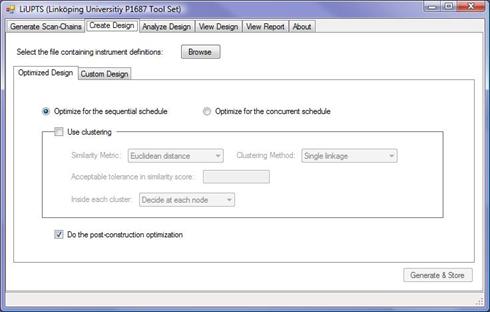
Figure 8 shows the options for construction of optimized designs.

To use this feature, the user selects the XML file containing the instruments list through the Browse button. The instrument list is an XML file having a structure similar to the one shown in Listing 8. After selecting the file, the name of the file is shown in the status bar and the “Generate & Store” button becomes enabled. After pressing the “Generate & Store” button, the “Save as” dialog appear asking for a file name to which the constructed network will be saved. The network will be saved in XML format having the structure described in Chapter 2. The generated XML file will then be shown in the “View Design” tab, as shown in Figure 9.

Listing 8

1: <?xml version="1.0"?>

2: <ScanChains>

3: <SIB ID="1" SCLength="297" SCPatterns="81" />

4: <SIB ID="2" SCLength="600" SCPatterns="84" />

5: <SIB ID="3" SCLength="773" SCPatterns="13" />

6: <SIB ID="4" SCLength="459" SCPatterns="37" />

7: <SIB ID="5" SCLength="54" SCPatterns="88" />

8: </ScanChains>

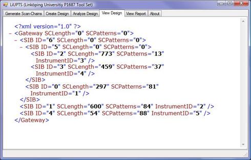
Figure 9 shows an XML file loaded into the View Design tab of LiUPTS user interface.

As can be seen in Figure 9, a new attribute/value pair named InstrumentID is added to each instrument SIB. The value for this attribute is taken from the ID attribute/value pair in the instrument list, see Listing 8. The InstrumentID attribute helps track that each of the instruments have ended up in which part of the constructed network.

Custom Design

To experiment with new IJTAG network construction algorithms, it might be useful to compare the results of those algorithms with some reference solutions to observe the improvements. These reference solutions can be relatively simple such as a network (made of the same instruments used by the proposed algorithms) having flat architecture or a hierarchical architecture in the form of a binary tree. When dealing with large number of instruments, creating such reference networks manually might be time consuming. The custom design feature of LiUPTS helps save time in construction of some reference networks. To use this feature select the “Create Design” tab and from within this tab select “Custom Design”. This feature is shown in Figure 10.

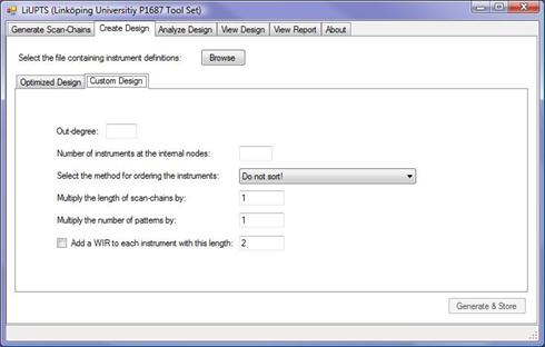
Figure 10: Random design construction feature

To use this feature, the user selects the XML file containing the instruments list through the Browse button. After selecting the file, the name of the file is shown in the status bar and the Generate & Store button becomes enabled. The type of architecture to be created is controlled through two parameters:

· Outdegree

· Number of instruments at the internal nodes

By using these two parameters, a variety of architectures can be obtained. For example, by setting both Outdegree and Number of instruments at the internal nodes to zero, an IJTAG network with flat architecture will be created. To construct a hierarchical design in the form of a binary tree where each node only accommodates one instrument SIB, Outdegree should be set to two and Number of instruments at the internal nodes should be set to one. If instead a binary tree is required where the instrument SIBs are only at the leaves and not the internal nodes, Outdegree should be set to two and Number of instruments at the internal nodes should be set to zero.

NOTE

Depending on the total number of instruments and the entered parameters, the tool tries to find the best hierarchical depth. But obviously it is not always possible to construct a fully balanced- i.e. symmetrical, structure.

The user can also tell the tool to sort the instruments list before the construction of the design. This feature might be useful, for example, when it is studied if the proximity of instruments with larger scan-chain lengths to the gateway has any effect on the average access time. The four possible sort types are:

· Sort by number of patterns in ascending order

· Sort by number of patterns in descending order

· Sort by length of scan-chains in ascending order

· Sort by length of scan-chains in descending order

It is also possible to scale up the number of patterns and scan-chain length of all instruments at the same time through “Multiply the length of scan-chains by” and “Multiply the number of patterns by” parameters. These will help study the results of a construction algorithm when the length and number of patterns properties of the instruments scale up.

Finally, it is possible to wrap all instruments in IEEE 1500 wrappers by checking the “Add a WIR to each instrument with this length” box and entering the length for the WIR.

NOTE

If a doorway SIB only has one child SIB on its HIP, the construction algorithm replaces that doorway SIB with the child SIB.

Figure 11 shows loading the instruments list in Listing 8, and Figure 12 shows the result after pressing the Generate & Store button (which asks for a file name to save the results). Note that the input parameters selected by user appear as XML comments in the design to help the user recall how the design is constructed.

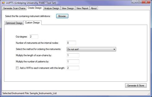
Figure 11 shows selecting the instrument file named Sample_Instruments_List and entering the desired parameters.

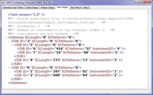
Figure 12 shows the created design.

Scan-chain Generation

In some experiments, for example when observing the performance of a network construction algorithm, it might be useful to generate a large list of instruments to be used in the study. LiUPTS provides the user with such a feature shown in Figure 13. The user specifies the number of scan-chains to be generated, as well as lower and upper bounds for randomly assigning length and number of patterns to each scan-chain. After pushing the Generate & Store button, the user will be prompted to enter a file name for storing the generated scan-chain list which is in XML format. Then the tool shows the generated file in the “View Design” tab as shown in Figure 14.

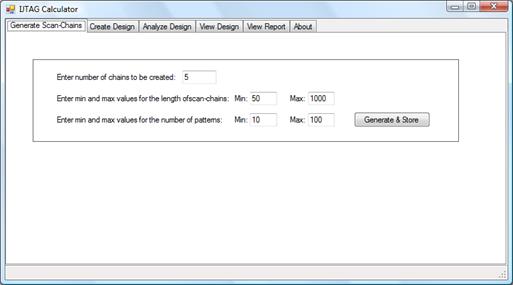
Figure 13: Scan-chain generation feature

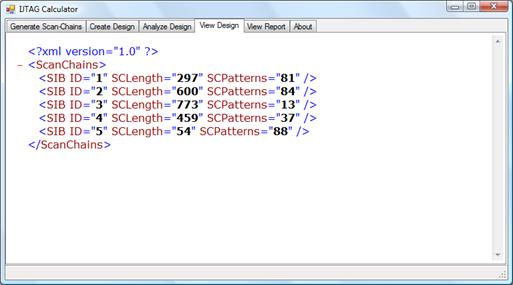
Figure 14: Randomly generated list of scan-chains

Appendix

Useful Material

The website of the IEEE P1687 working group [4] contains a series of presentation made by the members of the group in a variety of seminars and workshops. Furthermore, the work in [1] gives an overview of how IJTAG works and how test time is to be calculated when instruments are scan-chains. Finally, the work in [2] discusses the construction of optimized P1687 networks.

Bibliography

[1]	Farrokh Ghani Zadegan, Urban Ingelsson, Gunnar Carlsson, and Erik Larsson, "Test Time Analysis for IEEE P1687," in IEEE 19th Asian Test Symposium (ATS2010), Shanghai, China, 2010.
[2]	Farrokh Ghani Zadegan, Urban Ingelsson, Gunnar Carlsson, and Erik Larsson, "Design Automation for IEEE P1687," in Design Autmation and Test in Europe (DATE 2011, Grenoble, France, 2011.
[3]	(2010, October) Microsoft Express downloads. [Online]. http://www.microsoft.com/express/Downloads/
[4]	IJTAG. [Online]. http://grouper.ieee.org/groups/1687/
[5]	Farrokh Ghani Zadegan, "Analysis and Optimization for Testing Using IEEE P1687," Linköping University, Linköping, Master Thesis LIU-IDA/LITH-EX-A--10/040--SE, 2010.
[6]	MJL de Hoon, S Imoto, Nolan, and S Miyano, "Open source clustering software," BIOINFORMATICS, vol. 20, no. 9, pp. 1453-1454, JUN 12 2004.