Localisation in an Uncertain World with Multiple Agents
Zheng Wang
Bernhard Hengst
Claude Sammut
School of Computer Science and Engineering
University of New South Wales
Sydney, Australia
Abstract
The information delivered by a robot's sensors always contains a high degree of uncertainty. When there are multiple communicating robots, there is an opportunity to combine sensor information to obtain a more complete model of the world. However, combining uncertain information in noisy and dynamic environments is fraught with many difficulties and can often make reasoning about the world more difficult. In this paper, we describe our attempts to combine world models of multiple robots in the RoboCup robot soccer domain. We work with Sony's Aibo legged robot. A team consists of four such robots, each of which operates autonomously, sensing its environment primarily through an onboard colour camera. Each robot is equipped with a wireless LAN card enabling it to communicate with its team mates. The robots attempt to localise themselves and other objects and construct a world model that may be shared. The problem we discuss is how the world models from other robots can be incorporated into a single model. We also discuss the dangers in attempting to do so.
1 Introduction
The purpose of the RoboCup competition is to stimulate research in advanced mobile robotics. For a mobile robot to operate effectively it must be capable of at least the following:
· perceive its environment through its sensors;
· use its sensory inputs to identify objects in the environment;
· use its sensors to locate the robot relative to other objects in the environment;
· plan a set of actions in order to achieve some goal;
· execute the actions, monitoring the progress of the robot with respect to its goal.
The robot's planning becomes much more complex when its environment includes other active agents, such as other robots. These may cooperate with the robot or try to thwart its attempts to achieve its goals.
A competitive game like soccer requires all of the above skills. Thus, RoboCup was created to provide an incentive for researchers to work, not only on the individual problems, but to integrate their solutions in a very concrete task. The benefits of the competition are evident in the progress from one year to the next. The competitive nature of the research has forced participants to evaluate very critically their methods in a realistic task as opposed to experiments in a controlled laboratory. It has also forced researchers to face practical hardware and real time constraints.
The Sony legged robot league is one of four leagues that currently form the RoboCup competition. In some leagues, the teams are required to design and build the robot hardware themselves. In the case of the Sony legged robot league, all teams use the same robotic platform, manufactured by Sony. The robots operate autonomously, meaning the robot is entirely on its own during the play of the game. Since all teams use the same hardware, the difference lies in the methods they devise to program the robots. Each team in the robot soccer match consists of four robots with the matches consisting of two 10-minute halves.
The robots used in the Sony legged league are a slightly modified version of the Sony Aibo entertainment robot. Although designed for the entertainment market, the Sony robots extremely sophisticated robots, with an on board MIPS R5000 processor, colour camera, accelerometers, contact sensors, speaker and stereo microphones. Each of the four legs has three degrees of freedom, as does the head. Programs are written in C++ using a PC-based development environment. Code is loaded onto a memory stick that is inserted into the robot.
The field used in the Sony legged league measures 3 metres wide by 4.5 metres long. The field has an angled white border designed to keep the ball within the field. The game ball is coloured orange and the two goals are coloured yellow and blue. The field also contains six coloured distinguishable landmark poles to aid the robots in localising themselves in the field. In front of each goal, is the penalty area, that only the goalie is allowed to defend. However, more than one attacker is allowed to enter the penalty area.
One of the most difficult tasks in creating the software to control the robots is localisation. That is, by observing landmarks around the field, the robot must be able to estimate its own position within the field and then estimate the positions of the ball and other robots. The source of difficulty in localisation is the inaccuracy of the sensors. The colour CMOS camera is the robot’s main sensor. Since the robot only has one camera, distance to a landmark is estimated by its apparent size. With an image resolution of only 196 x 144 pixels, distant objects may occupy only a few pixels, so a difference of one or two pixels can make a big difference to the distance estimate. Noise in the camera image almost guarantees that there will be pixels that appear the incorrect colour and therefore the size of the object and therefore its distance is always uncertain. So the question is: how can the robot function reasonably reliably with uncertain sensors.
In 2002, a new addition to the competition was the availability of wireless network communication between the robots. This allows robots to share information about the world. In theory, one would think that this is a good idea since, for example, a robot that is unable to see the ball may still know its location because a team mate that can see the ball can broadcast its world model. Suppose however that two robots can see the ball, but due to the inaccuracy of their sensors, each has a different estimate of the ball’s location. Which should be believed? Can two uncertain measurements be combined sensibly? In this paper, we address these problems and describe our experiences in attempting to solve them for a domain that contains eight autonomous robot interacting and interfering with each other in often unpredictable ways.
2 Localisation
Information from the robot’s vision system, as well as odometry from the locomotion module, are combined to create a world model. Since the dimensions of the field are known in advance, the world model is constructed by placing the mobile objects on a map of the field. As objects are observed to move, their positions in the map are updated. However, some apparent motions may only be due to noise in the image. It is therefore unwise to instantaneously update the position based on a single measurement.
Until the 2002 competition, the update method adopted was to compromise between the objects current position in the world model and the perceived position by gradually “nudging” the position away from the current position towards the perceived position. An ad hoc confidence factor was attached to the location of an object in the world model. This described a belief in the accuracy of the estimated distance to the object. The confidence factor was based on the percentage of the object seen and other criteria. It was used to determine the weight of the contribution of the object’s perceived distance to the update of the estimated position of the object. The update algorithm is described in Figure 1.
r = gain 0 ≤ r ≤ 1
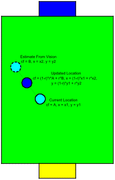
Figure 1, Old World Model Location Update
Figure 1 shows the general concept of the old world model. The gain is applied to adjust the speed of updates.
This localization method worked well in previous competitions. However, in 2002 the size of the field was increased from 2 x 3 metres to 3 x 4.4 metres. This meant that the measurements to distant objects became even more unreliable than before and the ad hoc method broke down. However, this method is a simple version of a more principled approach to updating sensor measurements, the Kalman Filter (Kalman, 1960).
3 The Kalman Filter
In the Kalman filter, there are two sets of equations: time update equations and measurement update equations (Welch and Bishop, 2001). The time update equations are responsible for projecting forward (in time) an estimated state, and are used when odometry information is received from the locomotion module. The measurement update equations on the other hand are responsible for feedback by incorporating new measurements and are used when information from the vision system is received. The two set of equations form an ongoing discrete Kalman filter cycle.
For the purposes of exposition, we will briefly explain how the Kalman filter works by describing how a robot can localise itself relative to fixed landmarks. The variables for robot localisation are the x and y coordinates, the variance of the location, the heading and the variance of the heading. The origin is at the bottom left corner of the field. The x‑axis runs along the edge of the field with the robot’s own goal below the axis and the opponents goal above the axis. The y-axis runs along the left edge of the field with the goals to the right of the axis.
Robot localisation uses beacons and goals as the landmarks and receives odometry from the locomotion module. When the robot sees a beacon or a goal, the identified object is passed to the world model. This module then uses the position measurements and the current estimated position and heading to build a new position and heading where it believes the robot should be. The robot first checks if it can see two beacons. If it can, it uses the two beacons to triangulate its location. If it can only see one beacon, it will use the Kalman Filter to move its estimated position towards the beacon so that the world model distance to the beacon is closer to the measured distance.
3.1 Measurement Update
Once, the distance and heading measurements are obtained, they must be combined with the current estimates of location and heading to derive the new state. At this point, the Kalman filter’s time measurement equations are applied. They are simplified for our task as:
![]()
![]()
![]()
where varx
is the measurement variance; R is
an estimate of the measurement noise (usually determined experimentally prior
to the measurements); K is called
the Kalman gain. First, the gain
and then the variance are updated. Assuming we are updating the estimate of the
x variable, we take the
difference, ![]() , of the current estimate and the measured value and use it
to adjust the estimate. The update equations above are repeated for the robot’s
y position and its heading. In
practice, we simplify the calculations further by assuming the x and y have
the same variance. The measurement noise, R, is calculated from the estimated distance of the
object since we know that the accuracy of the distance measurement becomes
worse as the size of the object in the image becomes smaller. This is discussed
further in Section 4.
, of the current estimate and the measured value and use it
to adjust the estimate. The update equations above are repeated for the robot’s
y position and its heading. In
practice, we simplify the calculations further by assuming the x and y have
the same variance. The measurement noise, R, is calculated from the estimated distance of the
object since we know that the accuracy of the distance measurement becomes
worse as the size of the object in the image becomes smaller. This is discussed
further in Section 4.
3.2 Time Update
The robot also uses the odometry measurements from the locomotion module to help it localise. This is useful because it allows the robot to know roughly where it is even when it has not seen a landmark for some time. However, its confidence in its location decreases very rapidly. To model this process, the Kalman filter’s time update equations are useful. Again, they are simplified to suit our task:
![]()
![]()
The measurement value, x, is simply updated by the displacement in x. The variance is updated by the process noise, Q. Q is estimated before hand. In the case of the legged robots, this is an experimentally determined estimate of the amount of slippage when the legs attempt to move the robot.
4 Vision System
To cater for Kalman filters the vision system must produce a variance measurement for each object identified. In order to escape from ad hoc values like the confidence factors, the variances of measurements are derived by recording the error in the estimated distance. By using statically collected variance measurements not only have we moved away from magic numbers, we have also made the confidence of distant measurement distant dependent. This means far objects will have much higher variance than those of closer objects due to the physical limitations of the camera. This should make the world model much more stable and resilient to error.
Estimated Distance (cm) Error in Distance Estimation
![]()
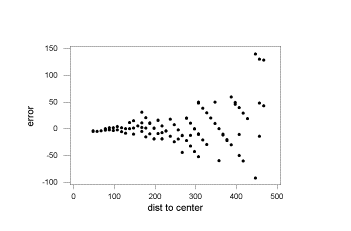
Figure 2. Error in Beacon Distance Estimation
To illustrate how the variance of distant measurements is
obtained we will demonstrate the process of constructing a variance equation
for beacons. First, a number of distance measurements are made for a beacon at
various distances. We have taken 450 samples for beacons. With the collected
data, we construct a graph (Figure
2),
which shows the behaviour of the error. By understanding the rough behaviour of
the error, we can determine how to model the variance. From this graph, we can
see the error increases over distance and in a logarithmic fashion. Hence, we
need a logarithm function to model the error. By finding a line of best fit for
the error, we can obtain the variance equation by simply squaring this line.
Next, to find the line of best fit, we take logs of the error and then apply
regression over the new values. Figure
3
shows the results of the regression. Finally, the equation for the variance of
beacons is obtained by taking the equation from regression, invert the log
function then square the result. The resultant equation for variance is ![]() .
.
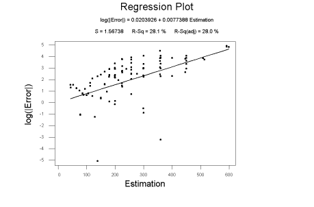
Figure 3, Regression Plot
With the above additions, the vision module is now able to produce a variance for each object recognised. In practice, because objects can be partially occluded or can be partially seen at the edge of the camera, the above variance is multiplied by a constant and divided by the percentage of the object seen. Though this seems to be fudging again, what is important is that a relationship between the distance of the observed object and its confidence is established.
5 Localising Other Objects
As well as localising itself, a robot must also estimate the positions of the ball and the other robots. The Kalman filter update algorithm is the same, however, an complication is added by the fact that there are several robots and it is not always obvious which robot position to update. Some heuristics to reduce this problem are described next.
5.1 Measurement Update
The Kalman filter uses variances to represent the confidence of object’s location. By assuming the error distribution is Gaussian we can say we are roughly confident the object should be with in a circle of radius 2s of the estimated location. s is the standard deviation and 2s corresponds to the 95% confidence interval for a Gaussian distribution. With this knowledge, we can find which robot to update by overlapping the Visual Model from the vision system with the World Model to find robots that have overlapping confidence regions. This process is illustrated in Figure 4.
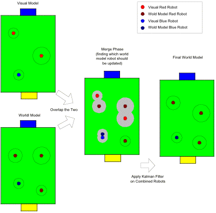
Figure 4. Updating Multiple Robot Locations
5.2 Time Update
To predict the next location of a ball or a robot must build a world model that records the direction and velocity of the object. Unfortunately, these measurements are difficult to obtain with the current sensors. Therefore, the time update in the Kalman filter algorithm is simulated by having an artificially high movement variance that assumes the object will move in any direction randomly. This time update simulation is carried out just before the measurement updates are carried out.
6 The Wireless Model
With the introduction of wireless communication between robots, a new level of representation, the wireless model, was added. This model is a representation of the world as given by a robot’s team mates. It is kept separate from the robot’s own world model. We associate with each team mate a variance which represents our confidence in the accuracy of the information from that robot. The variance of an object in the wireless model is the sum of the team mate’s variance, the object’s variance, as believed by the team mate, and a small variance for the latency over the wireless network.
During a game, each robot on the field receives information from every other robot. This means that a robot must combine the world models of all three other robots and its own. The technique is the same as shown in Figure 4, except in this case the inputs will be four world models, one for each team mate. Where the variances of two robots overlap, they are combined into one. The equation for how the information of the two robots is merged is shown in the following pseudo code.
result.x = (robot1.x*robot1.var +
robot2.x*robot2.var)/(robot1.var + robot2.var)
result.y = (robot1.y*robot1.var +
robot2.y*robot2.var)/(robot1.var + robot2.var)
result.var = 2*( robot1.var* robot2.var)/( robot1.var + robot2.var)
Once the information is merged, the best (lowest variance) four robots of each colour are stored in the wireless model. The same process is also applied to combine information for balls. In this case, only the best ball is selected. In the wireless model, three extra robots are also stored. These describe the location of the team mates according to their own belief.
7 Evaluation
An evaluation of the localisation method can be done in terms of accuracy, responsiveness and robustness.
7.1 Accuracy
It is interesting to compare the old ad hoc method for localisation versus the new method based on the Kalman Filter. One robot was programmed with the old method and another with the new. Both were placed in the same location. The robots constantly panned their heads, searching for landmarks. The behaviour of the old world model is excellent when it is looking at nearby beacons. However, once it is at one end of the field and facing the other end, its estimated position in the world model jumps erratically. This is because of the old world model assumes that beacon distance measurement is always accurate. That is, the error estimate functions are not distant dependent. When the new world model is used, it has similar problems. However, it is much steadier. Thanks to Kalman filters, it is possible to adjust the steadiness of the world model by tuning a few parameters, such as the process noise, Q. Figure 5 shows a comparison of the two world models. We can see that the old world model has a greater scatter of position estimates.
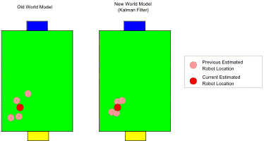
Figure 5, World Model Comparison
The introduction of wireless communication in the 2002 competition meant that the robots could share their world models. Theoretically, this means that a robot should be play blind folded, as long as the other robots because it can maintain a world model based on the observations of the other robots. In practice, however, it is not so simple. Although, the wireless model incorporates information from all robots, it has the deficiency that because every robot has its own errors in localisation, the resultant wireless model is useful only for coarse-grained behaviours such as getting to a far ball and avoiding interfering with a team mate. In fine-grained behaviours, such as kicking a ball, which needs accuracy to the centimetre, the wireless model is too noisy. To demonstrate this, Figure 6 shows the result of overlapping the world models of two robots. For simplicity, the world models only contain the ball. The purpose of this demonstration is to show how small errors between the world models of two different robots can greatly affect the final model. Note that both robots have slightly inaccurate estimates of the ball’s position. When the estimates are combined, the new ball position is not an improvement.
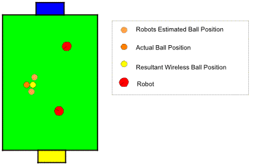
Figure 6, Wireless Model Limitations
7.2 Responsiveness
Responsiveness is a measure of how fast a robot reacts to new information. That is, how fast is the world model accurately updated? The faster the update, the more reactive is the system. There is a trade off because a robot tat responds too quickly to new information will be seriously affected by noise. Once again, by tuning a few parameters it is possible to adjust for this trade off. This was more difficult with the old world model because the variance of a landmark mainly depended on the percentage of the object seen and not its distance.
Observations of these behaviours were made during game play. Wireless communication allowed each robot to transmit its world model to a base station where real-time graphical display enabled us to capture that world model updates. When the beacons were a long way from the robot, they might appear only as tall as 7 or 8 pixels. With a lot of noise, “ghost beacons” could also appear. Under the old world model, the robots would occasionally “teleport” across field then back, causing erratic behaviours. With the new world model, the robots quickly responded to nearby beacons and responded quickly to far beacons only no other landmark had been seen for a long time.
7.3 Robustness
The vision system recognises objects by forming blobs of pixels, all of the same colour. As mentioned previously, distant objects may form blobs containing only a few pixels and thus are difficult to distinguish from noise. A simple remedy is to reject blobs that are smaller than some threshold value. If the threshold is set too high, we risk throwing away useful information. If it is set to low, we risk creating many phantom objects in the world model. This problem was reduced somewhat because we collected statistics on the noise in the data, which could be incorporated into the Kalman filter.
8 Conclusion
Despite the many improvements obtained through the use of a principled technique such as the Kalman Filter. Localisation remains a difficult problem. Erratic positioning and frequent errors can be reduced somewhat, but not eliminated. Combining information from other robots can be of use on some occasions, but in others situations, it is better to ignore the information coming from team mates and rely on onboard sensors. For these reasons, the game play software contains many heuristics that attempt to use “common sense” in the application of localisation techniques. Unfortunately, the heuristics are also ad hoc and prone to error. Ideally, one would like to be able to place robots on the field and have them learn to tune parameters and acquire or discard heuristics. When dealing with physical systems, however, one cannot afford to run the thousands of trials often required by learning systems and, so far, learning in simulation has not transferred well to the physical world. Thus, many challenges remain in finding effective methods for dealing with uncertainty and noise in physical systems.
References
Kalman, R. E. (1960). A New Approach to Linear Filtering and Prediction Problems, Transactions of the ASME – Journal of Basic Engineering, 82(D), 35-45.
Welch, G. and Bishop, G. (2001). An Introduction to the Kalman Filter, TR 95-041, Department of Computer Science, University of North Carolina at Chapel Hill, Chapel Hill, NC 27599-3175, February 8, 2001.