ModelicaAdditions.MultiBody

Information

This library is used to model 3-dimensional mechanical systems, such as robots, satellites or vehicles. The components of the MultiBody library can be combined with the 1D-mechanical libraries Modelica.Mechanics.Rotational and Modelica.Mechanics.Translational. A unique feature of the MultiBody library is the efficient treatment of joint locking and unlocking. This allows e.g. easy modeling of friction or brakes in the joints.

A first example to model a simple pendulum is given in the next figure:

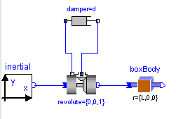
This system is built up by the following components:

• Component inertial is an instance of MultiBody.Parts.InertialSystem and defines the inertial system of the model as well as the gravity acceleration
• Component revolute is an instance of MultiBody.Joints.Revolute and defines a revolute joint which is connected to the inertial system. The axis of rotation is defined to be vector {0,0,1}, i.e., a vector in z-direction resolved in the frame at the left side of the revolute joint. Since this frame is rigidly attached to the inertial frame, these two frames are identical. As a consequence, the revolute joint rotates around the z-axis of the inertial system.
• Component boxBody is an instance of MultiBody.Parts.BoxBody and defines a box. The box is defined by lenght, width and height and some material properties, such as the density. The mass, center of mass and inertia tensor are calculated from this data. Additionally, the shape of the box is used for animation.
• Component damper is an instance of Modelica.Mechanics.Rotational.Damper and defines the velocity dependent damping in the joint axis. It is connected between the driving flange axis of the joint and flange bearing. Both flanges are 1D mechanical connections.

The 3D-components are connected together at connectors Frame_a or Frame_b. Both connectors define a coordinate system (a frame) at a specific location of the component, which is fixed in the component. The frame, i.e., the corresponding connector, is defined by the following variables:

  S[3,3]: Rotation matrix describing the frame with respect to the inertial
          frame, i.e. if ha is vector h resolved in frame_a and h0 is
          vector h resolved in the inertial frame, h0 = S*ha.
  r0[3] : Vector from the origin of the inertial frame to the origin
          of the frame, resolved in the inertial frame in [m] !!! (note,
          that all other vector quantities are resolved in frame_a!!!).
  v[3]  : Absolute (translational) velocity of the frame, resolved in
          the frame in [m/s]:  v = transpose(S)*der(r0)
  w[3]  : Absolute angular velocity of the frame, resolved in the frame,
          in [rad/s]:  w = vec(transpose(S)*der(S)), where
                      |   0   -w[3]  w[2] |
            skew(w) = |  w[3]   0   -w[1] | and w=vec(skew(w)) 
                      | -w[2]  w[1]   0   |
  a[3]  : Absolute translational acceleration of the frame minus gravity
          acceleration, resolved in the frame, in [m/s^2]:
             a = transpose(S)*( der(S*v) - ng*g )
          (ng,g are defined in model MultiBody.Parts.InertialSystem).
  z[3]  : Absolute angular acceleration of the frame, resolved in the 
          frame, in [rad/s^2]:  z = transpose(S)*der(S*w)
  f[3]  : Resultant cut-force acting at the origin of the frame,
          resolved in the frame, in [N].
  t[3]  : Resultant cut-torque with respect to the origin of the frame,
          resolved in the frame, in [Nm].

If two frame-connectors are connected together, the corresponding frames are rigidly fixed together, i.e., they are identical. Usually, all vectors of a component are expressed in frame_a of this component, i.e., in a coordinate system fixed in the component. For example, the vector from the origin of frame_a to the center-of-mass in component MultiBody.Parts.Body is resolved in frame_a.

Similiarily to the pendulum example above, most local frames are parallel to each other, if the generalized relative coordinates of the joints are zero. This means that in this configuration all vectors can be defined, as if the vectors would be expressed in the inertial frame (since all frames are parallel to each other). This view simplifies the definition. Only, if components Parts.FrameRotation, Parts.FrameAxes or Parts.FrameAngles are used, the frames are no longer parallel to each other in this nominal configuration.

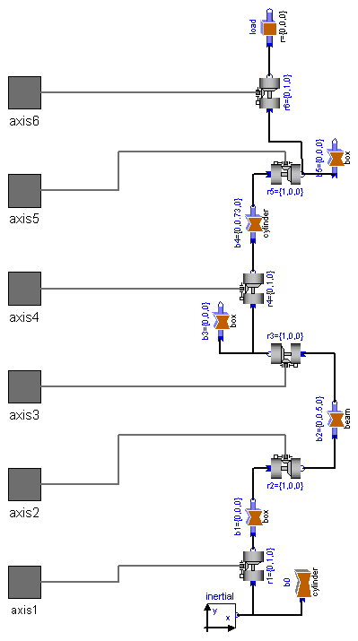
A more advance example is shown in the next figure. It is the definition of the mechanical structure of the robot r3, defined in the MultiBody.Examples.Robots.r3 sublibrary. It consists of a robot with 6 degrees-of-freedoms constructed with 6 revolutes joints and 6 shape bodies (i.e., the mass and inertia data is computed from shape data). The flanges of the driving axes of the joints are defined as flanges external to the model (connectors axis1, axis2, ..., axis6).

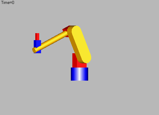
After processing the r3 model with a Modelica translator and simulating it, an animation can be performed:

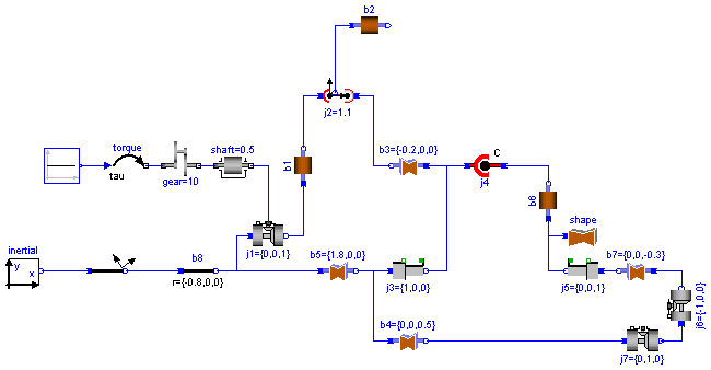
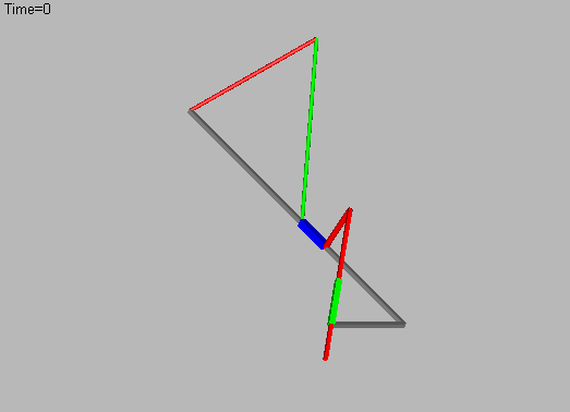
It is also possible to define multibody systems which have kinematic loops. An example is given in the next two figures (as object diagram and as animation view) where a mechanism with two coupled loops and one degree of freedom is shown:

The ModelicaAdditions.MultiBody library consists of the following elements:

• Inertial system (in package MultiBody.Parts):
  Exactly one inertial system must be present.
• Rigid bodies in package MultiBody.Parts (grey icons or brown icons if animation information included):
  There are several model classes to define rigid bodies which have mass and inertia. Often it is most convienient to use the BoxBody- and CylinderBody-model classes. Here, a box or a cylinder is defined. From the definition the mass, center of mass and inertia tensor is computed. Furthermore, the defined shape is used in the animation. All body objects have at most 2 frames where the body can be connected with other elements. If a rigid body has several attachment points where additional elements can be connected, it has to be built up by several body or (massless) frame elements (FrameTranslation, FrameRotationm ...) which are rigidly connected together. Presently, elastic bodies are not supported.
• Joints in the spanning tree in package MultiBody.Joints:
  A general multibody system with closed kinematic loops is handeled by dividing the joints into two distinct sets: Tree-Joints and Cut-Joints. After removal of all of the Cut-Joints, the resulting system must have a tree-structure. All joints in subpackage Joints, are joints used in this spanning tree. The relative motion between the two cut-frames of a Joint is described by f (0 <= f <= 6) generalized minimal-coordinates q and their first and second derivatives qd, qdd. By default, q and qd are used as state variables. In a kinematic loop, 6-nc degrees-of-freedom have to be removed, when the cut-joints introduces nc constraints. The Modelica translator can perform this removal automatically. In order to guide the translator, every joint has a parameter startValueFixed which can be used to require, that a particular degree-of-freedom should be selected as a state, because the given start values for the generalized coordinates q and qd have to be taken literally (this is realized, by setting attribute fixed = startValueFixed for the corresponding potential state variables). The one-degree-of-freedom joints (Revolute, Prismatic, Screw) may have a variable structure. That is, the joint can be locked and unlocked during the movement of a multibody system. This feature can be used to model brakes, clutches, stops or sticking friction. Locking is modelled with elements of the Modelica.Mechanics.Rotational library, such as classes Clutch or Friction, which can be attached to flange axis of the joints.
• Cut-Joints in package MultiBody.CutJoints:
  All red joints are cut joints. Cut joints are used to break closed kinematic loops (see previous paragraph).
• Force elements in package MultiBody.Forces:
  Force elements, such as springs and dampers, can be attached between two points of distinct bodies or joints. However, it is not possible to connect force elements with other force elements. It is easy for an user to introduce new force elements as subclasses from already existing ones (e.g. from model class MultiBody.Interfaces.LineForce). One-dimensional force laws can be used from the MultiBody.Mechanics.Rotational library. Gravitational forces for all bodies are taken into account by setting the gravitational acceleration of the inertial system (= object of MultiBody.Parts.InertialSystem) to a nonzero value.
• Sensor elements in package MultiBody.Sensors (yellow icons):
  Between two distinct points of bodies and joints a sensor element can be attached. A sensor is used to calculate relative kinematic quantities between the two points. In the libraries a general 3D sensor element (calculate all relative quantities) and a line-sensor element are present.

Connection Rules:
The elements of the multibody library cannot be connected arbitrarily together. Instead the following rules hold:

1. Tree joint objects, body objects and the inertial system have to be connected together in such a way that a frame_a of an object (cut filled with blue color) is always connected to a frame_b of an object (non-filled cut). The connection structure has to form a tree with the inertial system as a root.
2. Cut-joint, force, and sensor objects have to be always connected between two frames of a tree joint, body or inertial system object. E.g., it is not allowed to connect two force objects together.
3. By using the input/output prefixes of Modelica in the corresponding connectors of the MultiBody library, it is guaranteed that only connections can be carried out, for which the library is designed.

This package is not part of the Modelica standard library, because a "truely object-oriented" 3D-mechanical library is under development. The essential difference is that the new library no longer has restrictions on connections and that the modeller does not have to handle systems with kinematic loops in a different way (as a consequence, sublibrary CutJoints will be removed; the structure of the remaining library will be not changed, only the implementation of the model classes).

Note, this library utilizes the non-standard function constrain(..) and assumes that this function is supported by the Modelica translator:

   Real r[:], rd[:], rdd[:];
      ...
   r   = ..
   rd  = ...
   rdd = ...
   constrain(r,rd,rdd);

where r, rd and rdd are variables which need to be computed somewhere else. Function constrain() is used to explicitly inform the Modelica translator that rd is the derivative of r and rdd is the derivative of rd and that all derivatives need to be identical to zero. The Modelica translator can utilize this information to use rd and rdd whenever the Pantelides algorithm requires to compute the derivatives of r. This enhances the efficiency considerably. A simple, but inefficient, implementation of constrain() is:

   r = 0;

In the multibody library, function contrain() is used in the cut joints, i.e., whenever kinematic loops are present.

References

The following paper can be downloaded from 
   http://www.dynasim.se/publications.html and

Algorithmic details of the multibody library are described in
    Otter M., Elmqvist H., and Cellier F.E:  Modeling of Multibody Systems
          with the Object-Oriented Modeling Language Dymola . Proceedings 
          of the NATO-Advanced Study Institute on  Computer Aided
          Analysis of Rigid and Flexible Mechancial Systems , Volume II, 
          pp. 91-110, Troia, Portugal, 27 June - 9 July, 1993. Also in:
          Nonlinear Dynamics, 9:91-112, 1996, Kluwer Academic Publishers.

Main Author:

Martin Otter
Deutsches Zentrum für Luft und Raumfahrt e.V. (DLR)
Institut für Robotik und Mechatronik
Postfach 1116
D-82230 Wessling
Germany
email: Martin.Otter@dlr.de

Release Notes:

• June 20, 2000 by Martin Otter:
  Realized.

Copyright (C) 2000, DLR.

The ModelicaAdditions.MultiBody package is free software; it can be redistributed and/or modified under the terms of the Modelica license, see the license conditions and the accompanying disclaimer in the documentation of package Modelica in file "Modelica/package.mo".