
7.2. The AVL Tree
The AVL tree (named for its inventors Adelson-Velskii and Landis) should be viewed as a BST with the following additional property: For every node, the heights of its left and right subtrees differ by at most 1. As long as the tree maintains this property, if the tree contains \(n\) nodes, then it has a depth of at most \(O(\log n)\). As a result, search for any node will cost \(O(\log n)\), and if the updates can be done in time proportional to the depth of the node inserted or deleted, then updates will also cost \(O(\log n)\), even in the worst case.
The key to making the AVL tree work is to alter the insert and delete routines so as to maintain the balance property. Of course, to be practical, we must be able to implement the revised update routines in \(\Theta(\log n)\) time.
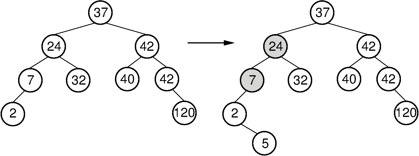
Figure 7.2.1: Example of an insert operation that violates the AVL tree balance property. Prior to the insert operation, all nodes of the tree are balanced (i.e., the depths of the left and right subtrees for every node differ by at most one). After inserting the node with value 5, the nodes with values 7 and 24 are no longer balanced.
Consider what happens when we insert a node with key value 5, as shown in Figure 7.2.1. The tree on the left meets the AVL tree balance requirements. After the insertion, two nodes no longer meet the requirements. Because the original tree met the balance requirement, nodes in the new tree can only be unbalanced by a difference of at most 2 in the subtrees. For the bottommost unbalanced node, call it \(S\), there are 4 cases:
- The extra node is in the left child of the left child of \(S\).
- The extra node is in the right child of the left child of \(S\).
- The extra node is in the left child of the right child of \(S\).
- The extra node is in the right child of the right child of \(S\).
Cases 1 and 4 are symmetrical, as are cases 2 and 3. Note also that the unbalanced nodes must be on the path from the root to the newly inserted node.
Our problem now is how to balance the tree in \(O(\log n)\) time. It turns out that we can do this using a series of local operations known as rotations. Cases 1 and 4 can be fixed using a single rotation, as shown in Figure 7.2.2. Cases 2 and 3 can be fixed using a double rotation, as shown in Figure 7.2.3.
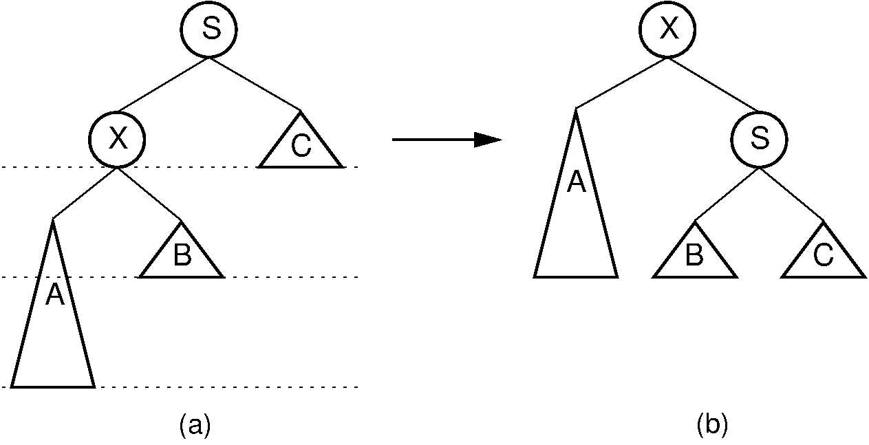
Figure 7.2.2: A single rotation in an AVL tree. This operation occurs when the excess node (in subtree \(A\)) is in the left child of the left child of the unbalanced node labeled \(S\). By rearranging the nodes as shown, we preserve the BST property, as well as re-balance the tree to preserve the AVL tree balance property. The case where the excess node is in the right child of the right child of the unbalanced node is handled in the same way.
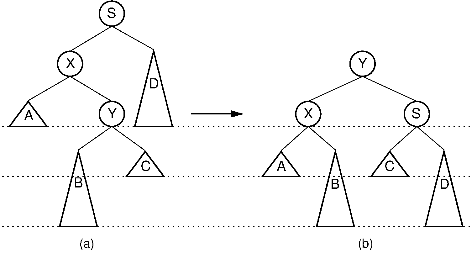
Figure 7.2.3: A double rotation in an AVL tree. This operation occurs when the excess node (in subtree \(B\)) is in the right child of the left child of the unbalanced node labeled \(S\). By rearranging the nodes as shown, we preserve the BST property, as well as re-balance the tree to preserve the AVL tree balance property. The case where the excess node is in the left child of the right child of \(S\) is handled in the same way.
The AVL tree insert algorithm begins with a normal BST insert. Then as the recursion unwinds up the tree, we perform the appropriate rotation on any node that is found to be unbalanced. Deletion is similar; however, consideration for unbalanced nodes must begin at the level of the deletemin operation.
Example 7.2.1
In Figure 7.2.1 (b), the bottom-most unbalanced node has value 7. The excess node (with value 5) is in the right subtree of the left child of 7, so we have an example of Case 2. This requires a double rotation to fix. After the rotation, 5 becomes the left child of 24, 2 becomes the left child of 5, and 7 becomes the right child of 5.